How to Build Your Retrieval-Augmented Generation (RAG)
These notes grew out of supervising student groups in 1DT104 Project in Computer Systems at Uppsala University, where the groups built a chatbot that answers questions about 3GPP telecom specifications using the TSpec-LLM dataset. I use that project as the running example throughout. The retrieval theory follows Manning, Raghavan, and Schütze’s “Introduction to Information Retrieval” and the RAG chapter of Jurafsky and Martin’s “Speech and Language Processing”.
How to Read These Notes
RAG is often taught as a recipe: “split your documents, embed them, put them in a vector database, stuff the top results into a prompt”. That recipe works on a demo and then fails in ways that are hard to debug, because each step hides a modelling decision. These notes take the slower route. We start from what a language model actually does, explain why it cannot be trusted with facts on its own, borrow the classical theory of information retrieval to understand search, and only then assemble the pipeline. Every metric comes with a worked numerical example so you can compute it by hand.
| Section | Question it answers |
|---|---|
| 1. What a language model knows | Why do we need retrieval at all? |
| 2. Classical retrieval | How does keyword search rank documents? |
| 3. Dense retrieval | How do embeddings find paraphrases? |
| 4. Measuring retrieval | How do we know if search works? |
| 5. The RAG architecture | How do the pieces fit together? |
| 6. Ingestion and chunking | How do raw documents become searchable units? |
| 7. The online retrieval stack | Hybrid search, fusion, reranking, packing |
| 8. Generation | Prompting, citations, abstention, conversation |
| 9. Advanced patterns | Which failure does each trick repair? |
| 10. Evaluating the whole system | Faithfulness, failure taxonomy, ablations |
| 11. Operating RAG | Latency, cost, freshness, security |
| 12. A minimal implementation | All of the above in about 100 lines of Python |
| 13. Project checklist | What I saw student groups get right and wrong |
The Running Example
The 3GPP specifications define how mobile networks (LTE, 5G NR) work. They are thousands of long, dense, cross-referencing documents, organized by series (TS 38.331 is the 5G radio resource control protocol, for example) and by release (Rel-15, Rel-16, Rel-17, …). A typical user question is:
What happens when timer T310 expires, and what starts it?
A general-purpose language model has probably seen some of this material during training, so it will produce a fluent answer. Whether the answer is correct, which release it refers to, and where it came from are exactly the questions RAG is designed to answer.
1. What a Language Model Knows, and What It Does Not
1.1 Next-Token Prediction
A large language model (LLM) is trained to predict the next token given the previous ones. For a token sequence $x_1,\ldots,x_T$ it models
\[p_\theta(x_1,\ldots,x_T)=\prod_{t=1}^{T}p_\theta(x_t\mid x_1,\ldots,x_{t-1}),\]where $\theta$ are billions of parameters fitted on a large text corpus. Generating an answer means repeatedly sampling (or picking the most likely) next token.
Everything the model “knows” is stored implicitly in $\theta$. Lewis et al. call this parametric memory. It has remarkable breadth, but it has four structural limitations.
- It is frozen. The parameters reflect the training data up to some cutoff date. A Rel-18 change published afterwards is invisible.
- It is public. The model has never seen your company’s internal documents, your course wiki, or a confidential design report.
- It is lossy on the long tail. Frequently repeated facts are memorized well; a timer value mentioned in one table of one specification is not.
- It has no provenance. The model cannot tell you where a fact came from, so you cannot check it.
1.2 Why Hallucinations Happen
The model is trained to produce plausible continuations, not true statements. When the relevant fact is well represented in training data, the plausible continuation and the true one coincide. When it is not, the model still produces a plausible continuation, because that is the only thing it knows how to do. The result is a confident, fluent, wrong answer: a hallucination. Asking the model to “be careful” does not change what it knows.
1.3 The Open-Book Exam
RAG changes the exam from closed-book to open-book. Before answering, we retrieve relevant passages from an external collection and place them in the prompt. The model now conditions on evidence:
\[\text{answer} \sim p_\theta(\,\cdot \mid \text{question},\ \text{retrieved passages}\,).\]The external collection is non-parametric memory: it can be updated by adding a document, restricted by access control, and cited in the answer. The language model’s job shifts from remembering to reading and synthesizing, which it is much better at.
Two consequences follow immediately and drive the rest of these notes:
- If the right passage is not retrieved, the model cannot use it. Most RAG failures are retrieval failures in disguise.
- Retrieved passages do not force the model to be faithful. The model can still ignore, misread, or over-generalize the evidence. Generation needs its own checks.
1.4 RAG, Fine-Tuning, or Long Context?
| Approach | What it changes | Good for | Weak at |
|---|---|---|---|
| Prompting only | nothing | general knowledge, style | private, recent, long-tail facts |
| Fine-tuning | model behaviour ($\theta$) | format, tone, domain vocabulary, task skills | adding many facts reliably; updating them; citing them |
| Long context | puts whole documents in the prompt | a few documents that fit | corpora larger than the window; cost per query; attention to the middle of long inputs |
| RAG | the evidence shown at inference time | large, changing, private corpora; provenance | questions needing a global view of the whole corpus |
These are complementary. A production system may fine-tune a model to follow a citation format and use retrieval to supply facts. For the 3GPP project, retrieval is unavoidable: the corpus is far larger than any context window, and users care which release a statement comes from.
What to Remember
- An LLM’s knowledge lives in its parameters: frozen, public, lossy, and unsourced.
- Hallucination is the model doing its job (plausible continuation) without the facts.
- RAG supplies evidence at inference time. Retrieval quality bounds answer quality.
2. Classical Retrieval: Ranking Documents by Words
Before embeddings, search engines ranked documents using word statistics. These methods are still in every serious RAG system, because they are fast, transparent, and excellent at exact identifiers like T310, PDCCH, or TS 38.331.
2.1 The Retrieval Problem
We have a corpus of $N$ documents (for RAG, usually chunks of documents) and a query $q$. We want a ranking: an ordered list of documents, most relevant first. “Relevant” means “useful for answering the information need behind the query”, which is a human judgment. A retrieval model is a scoring function $\mathrm{score}(q, d)$ that we hope correlates with that judgment.
2.2 The Inverted Index
Scanning every document for every query is too slow. The fundamental data structure of search is the inverted index: for each term, the list of documents containing it (its postings list).
Take three tiny documents:
d1: timer T310 radio link failure
d2: radio link monitoring out of sync
d3: handover timer T304
The inverted index is
failure    -> d1
handover   -> d3
link       -> d1, d2
monitoring -> d2
of         -> d2
out        -> d2
radio      -> d1, d2
sync       -> d2
t304       -> d3
t310       -> d1
timer      -> d1, d3
To answer the Boolean query radio AND link, intersect the postings lists of radio and link: $\lbrace d1, d2\rbrace$. Intersection of sorted lists takes time linear in their lengths, independent of corpus size. This is why search over billions of web pages is possible.
Boolean retrieval gives a set, not a ranking. To rank, we need weights.
2.3 Term Frequency and Inverse Document Frequency
Two intuitions:
- Term frequency (tf). A document that mentions the query term often is more likely about it. Let \(\mathrm{tf}_{t,d}\) be the number of occurrences of term $t$ in document $d$.
- Inverse document frequency (idf). A term that appears in almost every document (like “the”, or “UE” in a 3GPP corpus) carries little information. A rare term (like “T310”) is highly discriminative. Let \(\mathrm{df}_t\) be the number of documents containing $t$; then
The tf-idf weight combines them, \(w_{t,d}=\mathrm{tf}_{t,d}\cdot\mathrm{idf}_t\), and the simplest ranking score sums the weights of the query terms:
\[\mathrm{score}(q,d)=\sum_{t\in q}\mathrm{tf}_{t,d}\cdot\mathrm{idf}_t.\]Worked example. Query: T310 radio link failure, on the three documents above ($N=3$).
| Term | $\mathrm{df}$ | $\mathrm{idf}=\log_{10}(3/\mathrm{df})$ |
|---|---|---|
| t310 | 1 | 0.477 |
| radio | 2 | 0.176 |
| link | 2 | 0.176 |
| failure | 1 | 0.477 |
Every term appears at most once per document, so tf is 0 or 1:
- $d1$: $0.477+0.176+0.176+0.477=1.306$
- $d2$: $0.176+0.176=0.352$
- $d3$: $0$
Ranking: $d1, d2, d3$. Notice how much the rare terms contribute: t310 alone outweighs radio and link together.
2.4 The Vector Space Model
We can view each document as a vector in a space with one dimension per vocabulary term, with entries $w_{t,d}$. The query is a vector too. Similarity is the cosine of the angle between them:
\[\cos(q,d)=\frac{q\cdot d}{\lVert q\rVert\,\lVert d\rVert}.\]Dividing by the norms removes the advantage of long documents, which have large vectors simply because they contain many words. Cosine similarity reappears unchanged in dense retrieval; only the vectors change.
2.5 BM25: The Workhorse
Raw tf has two problems. First, the tenth occurrence of a term is much less informative than the first; relevance saturates. Second, long documents have more occurrences of everything. Okapi BM25 fixes both:
\[\mathrm{BM25}(q,d)=\sum_{t\in q}\mathrm{idf}_t\cdot \frac{\mathrm{tf}_{t,d}\,(k_1+1)}{\mathrm{tf}_{t,d}+k_1\left(1-b+b\,\dfrac{\lvert d\rvert}{\mathrm{avgdl}}\right)},\]where $\lvert d\rvert$ is document length, $\mathrm{avgdl}$ is the average length, and typical parameters are $k_1\approx 1.2$, $b\approx 0.75$. A common idf variant is \(\ln\left(\frac{N-\mathrm{df}_t+0.5}{\mathrm{df}_t+0.5}+1\right)\).
Let us see what the fraction (the tf component) does, with $k_1=1.2$, $b=0.75$.
Saturation (document of average length, so the bracket equals 1):
| tf | tf component |
|---|---|
| 1 | $\frac{1\cdot 2.2}{1+1.2}=1.000$ |
| 2 | $\frac{2\cdot 2.2}{2+1.2}=1.375$ |
| 10 | $\frac{10\cdot 2.2}{10+1.2}=1.964$ |
| $\infty$ | $\to k_1+1=2.2$ |
Going from one to two occurrences helps; going from ten to a hundred barely does. The parameter $k_1$ controls how fast saturation sets in.
Length normalization (tf = 1, document twice the average length): the bracket is $1-0.75+0.75\cdot 2=1.75$, so the component is $\frac{2.2}{1+1.2\cdot1.75}=\frac{2.2}{3.1}=0.710$. The same single mention counts less in a long document. The parameter $b$ controls how strongly length is penalized ($b=0$ turns it off).
BM25 has been a strong baseline for decades. In the BEIR benchmark (Thakur et al.), which tests retrievers on domains they were not trained on, BM25 remains competitive with many neural retrievers. For technical corpora full of identifiers, that matters.
2.6 Text Processing Choices
Keyword search depends on how text is split into terms:
- Tokenization. Is
T310one term? Isout-of-syncone term or three? Is38.331a number to keep intact? Technical corpora need tokenizers that preserve identifiers. - Case folding. Usually lowercase everything.
- Stop words. Very frequent words are often removed; BM25’s idf already down-weights them, so removal matters less than it used to.
- Stemming/lemmatization. Map “failures”, “failed”, “failing” to a common stem. Helps recall in prose; can hurt precision for identifiers.
What to Remember
- The inverted index makes keyword search fast.
- tf rewards repetition, idf rewards rarity; BM25 adds saturation ($k_1$) and length normalization ($b$).
- Keyword retrieval is precise on exact terms and identifiers, and robust on new domains.
3. Dense Retrieval: Searching by Meaning
3.1 The Vocabulary Mismatch Problem
Keyword methods fail when the query and the relevant passage use different words. A user asks “what happens when the phone loses the signal for too long?”; the specification says “upon expiry of T310, the UE shall consider radio link failure to be detected”. There is almost no word overlap. Lexical scores will be low, even though the passage answers the question.
3.2 Embeddings
A text embedding model $f$ maps a piece of text to a vector in $\mathbb R^d$ (typically $d$ between 384 and 4096) such that texts with similar meaning land near each other. Retrieval becomes nearest-neighbour search:
\[\mathrm{sim}(q,c)=\cos\big(f(q),f(c)\big)=\frac{f(q)\cdot f(c)}{\lVert f(q)\rVert\,\lVert f(c)\rVert}.\]If all vectors are normalized to unit length, cosine similarity equals the dot product, which is what vector indexes compute fastest.
A toy example in three dimensions. Suppose $f(q)=(0.8,0.6,0)$, $f(c_1)=(0.6,0.8,0)$ and $f(c_2)=(0,0.6,0.8)$, all unit length. Then $\cos(q,c_1)=0.48+0.48=0.96$ and $\cos(q,c_2)=0.36$. Chunk $c_1$ is retrieved first. Real embeddings have hundreds of dimensions, but the geometry is the same.
3.3 Bi-Encoders and Cross-Encoders
There are two ways to use a neural network to score query-passage pairs.
Bi-encoder. Encode query and passage separately, then compare vectors. Passage vectors can be computed once, offline, and stored. At query time we encode only the query and search the index. This scales to millions of passages.
Cross-encoder. Feed the query and passage together into one network, which outputs a relevance score. The network can attend across both texts, so it is much more accurate, but nothing can be precomputed: scoring $k$ passages needs $k$ forward passes per query.
The standard design uses both: a bi-encoder (and BM25) retrieves a few hundred candidates quickly, then a cross-encoder reranks the top candidates. Section 7 returns to this.
3.4 How Embedding Models Are Trained
Dense retrievers such as DPR (Karpukhin et al.) are trained with a contrastive loss. Given a query $q$, a relevant passage $p^{+}$, and a set of other passages $p_1,\ldots,p_n$ (often the positives of other queries in the same batch, called in-batch negatives), minimize
\[\mathcal L=-\log\frac{\exp\big(s(q,p^{+})/\tau\big)}{\exp\big(s(q,p^{+})/\tau\big)+\sum_{j=1}^{n}\exp\big(s(q,p_j)/\tau\big)},\]where $s$ is the similarity and $\tau$ a temperature. This is a softmax classification: “which of these passages is the right one?”. It pulls matching pairs together and pushes others apart. Hard negatives, passages that look relevant but are not (for example, high BM25 scores without the answer), make training much more effective.
The practical consequence: an embedding model is only as good as the notion of “similar” it was trained on. A general-purpose model may consider “T310” and “T311” nearly identical, because they appear in similar contexts. For identifier-heavy questions, that is a bug.
3.5 Dense Versus Sparse
| Sparse (BM25) | Dense (embeddings) | |
|---|---|---|
| Matches | exact terms | meaning, paraphrase |
| Identifiers, codes, names | strong | often weak |
| Synonyms, natural phrasing | weak | strong |
| New domain without training | robust | can degrade |
| Interpretability | high (which terms matched) | low |
| Index | inverted index | vector index |
Because their failure modes differ, combining them (hybrid retrieval, section 7) is usually better than either alone.
3.6 Nearest-Neighbour Search at Scale
Exact search compares the query with every stored vector: $N$ dot products of dimension $d$. For one million chunks with $d=768$ in 32-bit floats, the index holds about $10^6\times768\times4\approx3$ GB and each query costs about $7.7\times10^8$ multiply-adds. That is still feasible on one machine with optimized matrix code. At hundreds of millions of vectors it is not, and we switch to approximate nearest neighbour (ANN) search, trading a little recall for large speedups.
- IVF (inverted file). Cluster the vectors with k-means. At query time, search only the
nprobeclusters whose centroids are closest. More probes, more recall, more time. - HNSW (hierarchical navigable small world graphs). Connect each vector to some near neighbours in a multi-layer graph. Search greedily walks the graph towards the query, starting from a coarse top layer. Very fast and accurate, memory-hungry.
- PQ (product quantization). Compress each vector by splitting it into sub-vectors and replacing each with the id of the nearest codebook entry. Distances are approximated from lookup tables. Saves memory, costs accuracy.
Every ANN index has knobs that trade recall against latency and memory. Measure the index’s recall against exact search on your own data before trusting it.
What to Remember
- Embeddings map text to vectors; retrieval becomes nearest-neighbour search under cosine similarity.
- Bi-encoders are fast and precomputable; cross-encoders are accurate and expensive. Use both, in stages.
- Dense retrieval finds paraphrases but can blur identifiers; sparse retrieval is the opposite.
- ANN indexes (IVF, HNSW, PQ) trade recall for speed and memory.
4. Measuring Retrieval
You cannot improve what you do not measure. Retrieval should be evaluated before the language model is involved, because the LLM can mask retrieval failures with plausible prose.
4.1 Test Collections
A retrieval test collection has three parts: the corpus, a set of queries, and relevance judgments stating which chunks are relevant to each query (binary, or graded such as 0-3). For the 3GPP project, a group can build one by:
- sampling chunks from the specifications;
- asking an LLM to write a question each chunk answers;
- having a person read each question-chunk pair, discarding bad ones and marking other chunks that also answer the question;
- adding real user questions as they arrive.
Fifty to a few hundred carefully checked questions are enough to compare design choices.
4.2 Precision and Recall at k
For one query, let the top-$k$ results be retrieved, and let $\mathrm{Rel}$ be the set of relevant chunks.
\[\mathrm{P@}k=\frac{\lvert\text{relevant in top }k\rvert}{k},\qquad \mathrm{R@}k=\frac{\lvert\text{relevant in top }k\rvert}{\lvert\mathrm{Rel}\rvert}.\]Worked example. Three chunks $A, B, C$ are relevant. The retriever returns, in order, $[A, X, B, Y, Z]$.
- $\mathrm{P@1}=1/1=1$, $\mathrm{P@5}=2/5=0.4$.
- $\mathrm{R@5}=2/3\approx0.667$.
For RAG, recall@k is usually the most important retrieval metric, where $k$ is the number of chunks you will actually put in the prompt. If the evidence is not in the top $k$, the generator never sees it. Precision matters second: irrelevant chunks waste context and can distract the model.
4.3 Mean Reciprocal Rank
When one good passage is enough, we care how early the first relevant result appears. The reciprocal rank is $1/\text{rank of first relevant result}$ (0 if none), and MRR averages it over queries.
Worked example. Query 1: first relevant at rank 1, so RR = 1. Query 2: first relevant at rank 3, so RR = 1/3. MRR = $(1+1/3)/2\approx0.667$.
4.4 Normalized Discounted Cumulative Gain
With graded relevance, nDCG rewards putting highly relevant results early. The discounted cumulative gain of a ranking with gains $g_1, g_2, \ldots$ is
\[\mathrm{DCG@}k=\sum_{i=1}^{k}\frac{g_i}{\log_2(i+1)},\]and nDCG divides by the DCG of the ideal ordering, so the result lies in $[0,1]$.
Worked example. Graded relevance of the five results: $[3,0,2,0,1]$.
\[\mathrm{DCG@5}=\frac{3}{1}+\frac{0}{1.585}+\frac{2}{2}+\frac{0}{2.322}+\frac{1}{2.585}=3+1+0.387=4.387.\]The ideal ordering is $[3,2,1,0,0]$:
\[\mathrm{IDCG@5}=\frac{3}{1}+\frac{2}{1.585}+\frac{1}{2}=3+1.262+0.5=4.762.\]So $\mathrm{nDCG@5}=4.387/4.762\approx0.921$.
What to Remember
- Build a small, human-checked test set early; it pays for itself many times.
- Recall@k (with $k$ = chunks in the prompt) is the key RAG retrieval metric.
- MRR measures how early the first hit appears; nDCG handles graded relevance.
5. The RAG Architecture
We can now assemble the system. RAG has two phases that share assumptions (chunking, metadata, embedding model) and must be designed together.
Offline (indexing). Collect documents, parse them, attach metadata, split into chunks, embed the chunks, and store vectors, text, and metadata in indexes.
Online (answering). Receive a question, possibly rewrite it, retrieve candidates (dense and sparse), filter and fuse them, rerank, pack the best into a prompt, generate an answer with citations, and log everything for evaluation.
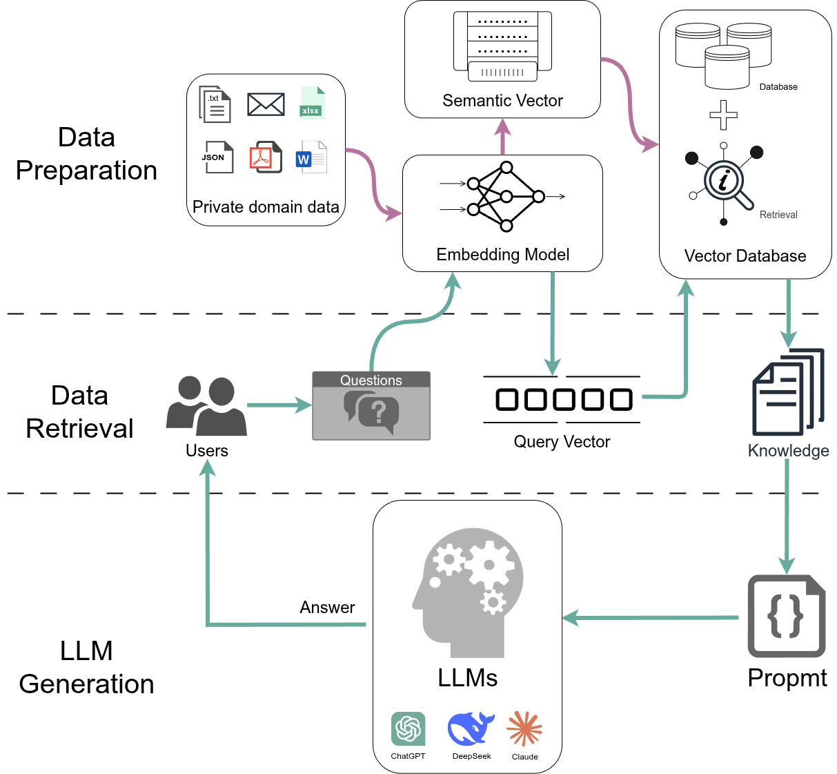

The original RAG model of Lewis et al. made this probabilistic. Let $z$ range over retrieved passages, with retriever probability $p_\eta(z\mid x)\propto\exp\big(f(z)^\top f(x)\big)$. RAG-Sequence uses one passage for the whole answer and marginalizes:
\[p(y\mid x)\approx\sum_{z\in\text{top-}k}p_\eta(z\mid x)\prod_{i}p_\theta(y_i\mid x,z,y_{1:i-1}).\]RAG-Token may switch passages at every token:
\[p(y\mid x)\approx\prod_{i}\sum_{z\in\text{top-}k}p_\eta(z\mid x)\,p_\theta(y_i\mid x,z,y_{1:i-1}).\]In that paper the retriever’s query encoder and the generator were trained jointly. Today’s RAG systems mostly use off-the-shelf retrievers and LLMs and simply concatenate retrieved passages into the prompt. The formulas still explain the essential structure: answer quality is an average over retrieval quality.
6. Ingestion: From Documents to Searchable Units

6.1 Parsing
Real documents are PDFs, Word files, HTML pages, spreadsheets, and scans. Parsing them into clean text is unglamorous and decisive. Typical problems:
- Headers, footers, and page numbers interleaved with body text (“3GPP TS 38.331 V17.x.x … Page 412”).
- Tables flattened into meaningless sequences of numbers. Timer values and parameter ranges in specifications live in tables.
- Multi-column layouts read in the wrong order.
- Figures and equations lost or garbled.
- Change marks and revision history mixed with normative text.
Before tuning anything else, open 20 random parsed chunks and read them. If you cannot answer a question from a chunk, neither can the model.
6.2 Metadata
Every chunk should carry metadata, because retrieval, filtering, citation, and access control all need it. An illustrative record for the 3GPP corpus:
{
  "chunk_id": "ts38331-r17-sec-rlf-003",
  "spec": "TS 38.331",
  "release": "Rel-17",
  "version": "17.x.x",
  "section": "Radio link failure related actions",
  "page": 412,
  "text": "...",
  "parent_id": "ts38331-r17-sec-rlf",
  "access": "public"
}
With this, the system can answer “according to Rel-16” by filtering on release, cite “TS 38.331, Radio link failure related actions”, and expand a small chunk to its parent section when needed.
6.3 Chunking
Embedding models accept limited input lengths, and a single vector cannot represent pages of varied content well. So documents are split into chunks. Formally, a document $D$ tokenized as $t_1,\ldots,t_n$ is covered by chunks $C_1,\ldots,C_m$ with $\lvert C_i\rvert\le L$.
The trade-off. Small chunks give precise vectors (one topic per vector) and precise retrieval, but may cut an answer in half or lose the context that makes a sentence meaningful (“it shall then start the timer”: which timer?). Large chunks keep context, but their vectors average over several topics and they consume more of the prompt budget.
Strategies:
- Fixed-size windows with overlap. Split every $L$ tokens, with $o$ tokens of overlap so a sentence near a boundary appears in both neighbours. Simple and robust.
- Recursive splitting. Try to split on section breaks, then paragraphs, then sentences, until pieces are under $L$.
- Structure-aware splitting. Use the document’s own structure: in specifications, numbered clauses are natural units. Prefix each chunk with its section heading path so it is self-describing.
- Semantic splitting. Start a new chunk where the embedding similarity between consecutive sentences drops.
Worked arithmetic for fixed windows. A section of $n=10{,}000$ tokens, $L=512$, $o=64$. The stride is $s=L-o=448$, and the number of chunks is
\[m=\left\lceil\frac{n-o}{s}\right\rceil=\left\lceil\frac{9936}{448}\right\rceil=\lceil 22.2\rceil=23.\]The index stores about $23\times512=11{,}776$ tokens, roughly 18% more than the original, the price of overlap.
A good default for technical documents: structure-aware splitting into chunks of a few hundred tokens, each prefixed with its document title and section path, plus a link to the parent section. Then measure recall@k on your test set with two or three chunk sizes and keep the best. Chunk size is a hyperparameter, not a law.
6.4 Parent-Child Indexing
A useful pattern decouples what you search from what you show. Index small child chunks (sentences or short paragraphs) for precise matching; when a child is retrieved, return its larger parent section to the model. A variant, “sentence window retrieval”, returns the matched sentence plus a few neighbours on each side.
6.5 Deduplication, Versions, and Updates
- Duplicates. Specifications repeat boilerplate; multiple releases repeat unchanged clauses. Near-duplicate chunks crowd out diverse evidence. Deduplicate at ingestion (hashing, or embedding similarity above a threshold), keeping release metadata.
- Versions. Decide whether the default answer uses the latest release and whether older releases are searchable on request.
- Updates. Track a content hash per document so re-ingestion only re-embeds what changed. If you change the embedding model, re-embed everything: vectors from different models are not comparable.
What to Remember
- Read your parsed chunks. Parsing errors are invisible downstream.
- Attach metadata (source, section, version, access) to every chunk.
- Chunk size trades precision against context; prefix chunks with headings; tune on recall@k.
- Search small, return big (parent-child). Deduplicate and version.
7. The Online Retrieval Stack

The online stack has a simple organizing principle: first stages maximize recall cheaply; later stages restore precision expensively.
7.1 Metadata Filtering
Apply hard constraints first: access permissions (never retrieve what the user may not see), release or date ranges, document types. Filtering before similarity search guarantees that the top-$k$ are all eligible; filtering after may leave you with too few results.
7.2 Hybrid Retrieval and Rank Fusion
Run BM25 and dense search in parallel, take the top 50-100 from each, and merge. The difficulty is that their scores are on incomparable scales (BM25 is unbounded; cosine lies in $[-1,1]$). Reciprocal Rank Fusion (RRF) sidesteps scores and uses only ranks:
\[\mathrm{RRF}(d)=\sum_{r\in\text{rankers}}\frac{1}{k+\mathrm{rank}_r(d)},\]with $k=60$ a common constant that dampens the influence of the very top ranks.
Worked example. BM25 returns $[d_3, d_1, d_7]$; dense search returns $[d_1, d_5, d_3]$.
| Document | BM25 rank | Dense rank | RRF score |
|---|---|---|---|
| $d_1$ | 2 | 1 | $\frac{1}{62}+\frac{1}{61}=0.03252$ |
| $d_3$ | 1 | 3 | $\frac{1}{61}+\frac{1}{63}=0.03226$ |
| $d_5$ | - | 2 | $\frac{1}{62}=0.01613$ |
| $d_7$ | 3 | - | $\frac{1}{63}=0.01587$ |
Fused ranking: $d_1, d_3, d_5, d_7$. Documents that both retrievers like rise to the top; a document found by only one retriever still survives.
7.3 Reranking
Take the top 20-50 fused candidates and score each (query, chunk) pair with a cross-encoder (section 3.3). Keep the top 3-10. Reranking is often the single most effective upgrade to a baseline RAG system, because it applies the most accurate model exactly where precision matters, on a small candidate set.
7.4 Diversity
If the top five chunks are near-copies of one clause from five releases, the prompt contains one piece of evidence five times. Maximal Marginal Relevance (MMR) selects chunks one at a time, balancing relevance against similarity to what has already been selected ($S$):
\[\mathrm{MMR}=\arg\max_{d\notin S}\Big[\lambda\,\mathrm{sim}(q,d)-(1-\lambda)\max_{d'\in S}\mathrm{sim}(d,d')\Big].\]With $\lambda=1$ this is plain relevance ranking; smaller $\lambda$ favours diversity.
7.5 Context Packing
The final step chooses what enters the prompt within a token budget. Suppose the model has a generous window, but cost and latency scale with input length. A typical budget: 300 tokens of instructions, 50 for the question, 6 chunks of about 500 tokens (3,000 tokens), and 500 reserved for the answer.
Two empirical observations guide packing:
- More is not always better. Irrelevant chunks dilute attention and can be quoted as if they were evidence.
- Position matters. Liu et al. (“Lost in the Middle”) found that models use information at the beginning and end of a long context more reliably than information in the middle. Put the strongest evidence first (or last), not buried in the middle.
What to Remember
- Filter first (permissions, versions), then retrieve broadly with BM25 and dense search.
- Fuse with RRF (rank-based, scale-free); rerank the top candidates with a cross-encoder.
- Enforce diversity (MMR, deduplication). Pack fewer, better chunks, strongest first.
8. Generation: Prompting for Grounded Answers
8.1 The Prompt Template
The prompt must tell the model how to use the evidence, not just provide it. A template that worked well for the student groups:
You are an assistant answering questions about 3GPP specifications.

Use ONLY the numbered sources below. For every factual statement,
cite the source number in square brackets, e.g. [2].
If the sources do not contain the answer, say so and state what is missing.
If sources disagree (for example, different releases), report both and
name the release of each.

Sources:
[1] (TS 38.331, Rel-17, Radio link failure related actions) ...
[2] (TS 38.331, Rel-17, Timers) ...
[3] ...

Question: What happens when timer T310 expires, and what starts it?

Answer:
The key elements:
- Role and scope (“questions about 3GPP specifications”).
- Grounding instruction (“use only the sources”).
- Citation format, with source ids that map back to chunk metadata, so the UI can link to the original text.
- Abstention rule: an explicit, acceptable way to say “not enough evidence”. Without it, the model will fill the gap from parametric memory.
- Conflict rule: what to do when sources disagree.
8.2 Why Citations Matter
Citations turn an answer from “trust me” into “check me”. They also make evaluation tractable: you can verify each cited claim against its source automatically or by hand (section 10). Ask for citations at the sentence or claim level, not one list at the end.
8.3 Decoding Settings
For factual question answering, use low temperature (near 0). Creativity is not wanted; consistency is. Limit answer length when the interface needs it.
8.4 Multi-Turn Conversations
Follow-up questions are often not searchable on their own: after asking about T310, a user asks “and what about T311?” or “does that change in Release 18?”. The fix is query condensation: before retrieval, have the LLM rewrite the latest message plus the chat history into a standalone query (“What is the role of timer T311 in TS 38.331?”), retrieve with that, and answer with the history plus new evidence.
What to Remember
- The prompt specifies grounding, citation, abstention, and conflict handling.
- Citations make answers checkable and the system evaluable.
- Low temperature for facts; condense conversational queries before retrieval.
9. Advanced Patterns, Organized by the Failure They Repair
A baseline pipeline (hybrid retrieval, reranking, good prompt) solves a surprising fraction of problems. Add advanced techniques only after error analysis shows which failure dominates. Each pattern below is listed with the failure it targets.

| Pattern | How it works | Failure it repairs |
|---|---|---|
| Query rewriting | LLM rephrases the user’s question in the corpus’s vocabulary | user phrasing differs from document phrasing |
| Multi-query | generate several phrasings, retrieve for each, fuse with RRF | a single query embedding misses relevant chunks |
| HyDE | LLM writes a hypothetical answer; embed that and search | short questions embed poorly; answers look like answers |
| Decomposition | split a compound question into sub-questions, retrieve each | “compare X in Rel-16 and Rel-17” needs two retrievals |
| Step-back prompting | also retrieve for a more general question | answer needs background the specific query misses |
| Routing | classify the question and send it to the right index or tool | one index cannot serve all question types |
| Parent-child / sentence window | match small, return larger context | retrieved chunk is too narrow to answer |
| Graph RAG | extract entities and relations; retrieve by graph traversal or community summaries | questions about relationships or the corpus as a whole |
| Tool use / agentic RAG | the model decides when to search, what to search, and when to stop | multi-step questions, structured data (SQL, APIs) |
A word of caution. Each extra LLM call adds latency, cost, and variance. An agentic pipeline with five LLM calls can be slower by seconds and harder to debug. In the student projects, the groups that improved the most were not those that added the most techniques, but those that built a test set and measured each change.
What to Remember
- Diagnose first; then pick the pattern that targets the dominant failure.
- Query-side fixes: rewriting, multi-query, HyDE, decomposition. Index-side fixes: parent-child, routing, graphs.
- Every orchestration step must earn its latency.
10. Evaluating the Whole System

10.1 Component Versus End-to-End
Evaluate retrieval and generation separately as well as together. If you only grade final answers, you cannot tell whether a wrong answer came from missing evidence or from misreading good evidence, and those need opposite fixes.
10.2 Generation Metrics
For each (question, retrieved context, answer) triple:
- Faithfulness (groundedness). Break the answer into atomic claims; the fraction of claims supported by the retrieved context. An unfaithful answer may still be true (from parametric memory), but it is unverifiable.
- Answer relevance. Does the answer address the question asked, completely and without padding?
- Context precision. Of the chunks given to the model, how many were actually useful?
- Context recall. Does the context contain everything a reference answer needs?
- Citation accuracy. Does each cited source actually support the sentence that cites it?
- Abstention quality. On questions the corpus cannot answer, does the system say so?
Frameworks such as RAGAS (Es et al.) automate these using an LLM as the judge.
10.3 Using LLMs as Judges, Carefully
LLM judges are cheap and scale, but they have biases: they prefer longer answers, answers in their own style, and the first of two options. Calibrate a judge by comparing its verdicts with human judgments on 50-100 examples before relying on it, and keep a human spot-check in the loop.
10.4 A Failure Taxonomy
Barnett et al. (“Seven Failure Points When Engineering a RAG System”) list where RAG systems break. Tagging each wrong answer in your test set with one of these tells you where to work:
- Missing content: the answer is not in the corpus. (Fix: corpus; abstention.)
- Missed top-ranked documents: the answer is in the corpus but not retrieved highly enough. (Fix: retrieval, chunking, hybrid, reranking.)
- Not in context: retrieved, but dropped during packing. (Fix: packing, budget.)
- Not extracted: in the context, but the model failed to use it. (Fix: prompt, ordering, less noise.)
- Wrong format: ignores the requested format. (Fix: prompt, structured output.)
- Incorrect specificity: too general or too detailed. (Fix: prompt, query understanding.)
- Incomplete: misses parts of the answer that were available. (Fix: decomposition, prompt.)
10.5 Ablations
Change one thing at a time and re-run the test set: chunk size, embedding model, BM25 on/off, reranker on/off, $k$, prompt version. Record recall@k, faithfulness, answer correctness, latency, and cost in a table. This is ordinary experimental science, and it is what separates engineering from guessing.
What to Remember
- Grade retrieval and generation separately.
- Faithfulness, answer relevance, context precision/recall, citation accuracy, abstention.
- Calibrate LLM judges against humans. Tag failures with a taxonomy; run ablations.
11. Operating a RAG System
11.1 Latency
A typical request budget: query embedding (tens of ms), vector and keyword search (tens of ms), reranking (around a hundred ms on a GPU for a few dozen pairs), LLM generation (often seconds, dominated by output length). LLM calls dominate, so every extra call (rewriting, multi-query, agents) is expensive. Stream the answer to the user to hide generation latency.
11.2 Cost
Cost scales with tokens: input tokens (prompt plus context) and output tokens, per request. Packing fewer, better chunks cuts cost and often improves quality. Cache embeddings of frequent queries and, where answers are stable, whole responses.
11.3 Freshness
Track which documents changed and re-index incrementally. Display the source version and date in answers. Periodically check for documents that failed to parse.
11.4 Security and Privacy
- Access control at retrieval time. Filter by the user’s permissions before retrieval. Never rely on the prompt (“do not reveal confidential documents”) as a security boundary.
- Indirect prompt injection. Retrieved documents are untrusted input. A document containing “ignore previous instructions and …” can hijack the model (Greshake et al.). Treat retrieved text as data: separate it clearly in the prompt, restrict what tools the model can call, and validate outputs.
- Logging. Logs of questions and answers are valuable for evaluation and may contain personal data; apply retention and anonymization rules.
11.5 Monitoring
Track in production: retrieval scores, the rate of “not enough information” answers, user feedback, latency percentiles, and cost per query. A sudden rise in abstentions often signals an ingestion failure; a drift in question topics signals missing content.
What to Remember
- LLM calls dominate latency and cost; tokens are the budget.
- Enforce permissions in retrieval, not in the prompt; treat retrieved text as untrusted.
- Monitor abstention rate, feedback, latency, cost, and index freshness.
12. A Minimal Implementation
The following is a complete, dependency-light pipeline: BM25 written from scratch, dense search with any embedding function, RRF fusion, and prompt assembly with citations. The LLM and embedding calls are left as functions so that the code does not depend on a particular provider.
import math
import re
from collections import Counter, defaultdict

import numpy as np


def tokenize(text):
    # Keep identifiers like t310 and 38.331 intact.
    return re.findall(r"[a-z0-9]+(?:\.[a-z0-9]+)*", text.lower())


def chunk_words(text, size=300, overlap=50):
    words = text.split()
    step = size - overlap
    return [" ".join(words[i:i + size])
            for i in range(0, max(len(words) - overlap, 1), step)]


class BM25:
    def __init__(self, docs, k1=1.2, b=0.75):
        self.docs = [tokenize(d) for d in docs]
        self.k1, self.b = k1, b
        self.N = len(self.docs)
        self.avgdl = sum(len(d) for d in self.docs) / self.N
        self.df = Counter(t for d in self.docs for t in set(d))
        self.tf = [Counter(d) for d in self.docs]

    def idf(self, t):
        n = self.df.get(t, 0)
        return math.log((self.N - n + 0.5) / (n + 0.5) + 1)

    def score(self, query_terms, i):
        dl = len(self.docs[i])
        norm = self.k1 * (1 - self.b + self.b * dl / self.avgdl)
        s = 0.0
        for t in query_terms:
            f = self.tf[i].get(t, 0)
            if f:
                s += self.idf(t) * f * (self.k1 + 1) / (f + norm)
        return s

    def search(self, query, k=50):
        terms = tokenize(query)
        scored = [(self.score(terms, i), i) for i in range(self.N)]
        scored.sort(reverse=True)
        return [i for s, i in scored[:k] if s > 0]


class DenseIndex:
    def __init__(self, docs, embed):
        self.embed = embed                      # embed(list[str]) -> np.ndarray
        vecs = embed(docs)
        self.vecs = vecs / np.linalg.norm(vecs, axis=1, keepdims=True)

    def search(self, query, k=50):
        q = self.embed([query])[0]
        q = q / np.linalg.norm(q)
        sims = self.vecs @ q                    # cosine similarity
        return list(np.argsort(-sims)[:k])


def rrf(rankings, k=60):
    scores = defaultdict(float)
    for ranking in rankings:
        for rank, doc in enumerate(ranking, start=1):
            scores[doc] += 1.0 / (k + rank)
    return sorted(scores, key=scores.get, reverse=True)


def build_prompt(question, chunks, metas):
    sources = "\n".join(
        f"[{n}] ({m['spec']}, {m['release']}, {m['section']}) {c}"
        for n, (c, m) in enumerate(zip(chunks, metas), start=1)
    )
    return (
        "Answer using ONLY the numbered sources. Cite sources like [1].\n"
        "If the sources do not contain the answer, say what is missing.\n\n"
        f"Sources:\n{sources}\n\nQuestion: {question}\nAnswer:"
    )


def answer(question, chunks, metas, bm25, dense, call_llm, n_ctx=6):
    fused = rrf([bm25.search(question), dense.search(question)])
    top = fused[:n_ctx]                         # add a reranker here
    prompt = build_prompt(question,
                          [chunks[i] for i in top],
                          [metas[i] for i in top])
    return call_llm(prompt), top
With this skeleton, each improvement from the earlier sections is a local change: swap chunk_words for structure-aware splitting, insert a cross-encoder between rrf and top, add a metadata filter before search, or wrap answer in a query-condensation step for conversations. Because answer returns the ids of the chunks used, you can compute recall@k and citation accuracy on your test set directly.
13. Project Checklist
This list collects what made the difference in the 1DT104 student projects.
Data
- Parsed text inspected by a human (tables, headers, multi-column pages).
- Metadata on every chunk: source, section path, version/release, page, access.
- Chunks prefixed with their heading path; parent links stored.
- Near-duplicates removed; versions handled deliberately.
Retrieval
- Test set of human-checked questions with relevant chunk ids.
- BM25 baseline measured before any dense model.
- Hybrid retrieval with RRF; reranker on the top candidates.
- Recall@k reported for the $k$ actually used in the prompt.
Generation
- Prompt specifies grounding, citations, abstention, and conflicts.
- Temperature low; output format fixed.
- Faithfulness and citation accuracy checked on the test set.
Operations
- Permissions enforced at retrieval time.
- Retrieved text treated as untrusted input.
- Latency and cost per query measured; logs retained responsibly.
The most common mistakes I saw:
- Judging the system by a handful of demo questions instead of a test set.
- Tuning prompts to fix what was actually a retrieval failure.
- Using only dense retrieval on a corpus full of identifiers (“T310” retrieving “T311”).
- Huge chunks “so the model has enough context”, which lowered recall@k and raised cost.
- Changing several components at once and not knowing which change helped.
Summary
| Layer | Core idea | Key metric |
|---|---|---|
| Language model | plausible continuation from parametric memory | - |
| Sparse retrieval | tf, idf, BM25 over an inverted index | recall@k, MRR |
| Dense retrieval | embeddings, cosine similarity, ANN | recall@k, nDCG |
| Ingestion | parsing, metadata, chunking, versions | chunk-level inspection |
| Retrieval stack | filter, hybrid, RRF, rerank, MMR, packing | recall@k at prompt size |
| Generation | grounding, citations, abstention | faithfulness, citation accuracy |
| System | failure taxonomy, ablations, monitoring | answer correctness, latency, cost |
RAG is not a truth machine. It is an evidence-routing architecture: it decides what the model gets to read. Most of the engineering is in making sure the right evidence arrives, and in checking that the model used it.
References and Reading Guide
- C. D. Manning, P. Raghavan, H. Schütze, Introduction to Information Retrieval (Cambridge, 2008). Chapters 1-2 (inverted index), 6 (tf-idf, vector space model), 8 (evaluation), 11 (probabilistic retrieval and BM25).
- D. Jurafsky, J. H. Martin, Speech and Language Processing (3rd ed. draft). Chapter on information retrieval, question answering, and RAG.
- P. Lewis et al., “Retrieval-Augmented Generation for Knowledge-Intensive NLP Tasks,” NeurIPS 2020.
- V. Karpukhin et al., “Dense Passage Retrieval for Open-Domain Question Answering,” EMNLP 2020.
- N. Thakur et al., “BEIR: A Heterogeneous Benchmark for Zero-shot Evaluation of Information Retrieval Models,” NeurIPS Datasets and Benchmarks 2021.
- G. V. Cormack, C. L. A. Clarke, S. Büttcher, “Reciprocal Rank Fusion Outperforms Condorcet and Individual Rank Learning Methods,” SIGIR 2009.
- J. Carbonell, J. Goldstein, “The Use of MMR, Diversity-Based Reranking for Reordering Documents and Producing Summaries,” SIGIR 1998.
- L. Gao et al., “Precise Zero-Shot Dense Retrieval without Relevance Labels” (HyDE), ACL 2023.
- N. F. Liu et al., “Lost in the Middle: How Language Models Use Long Contexts,” TACL 2024.
- S. Es et al., “RAGAS: Automated Evaluation of Retrieval Augmented Generation,” EACL 2024 (demo).
- S. Barnett et al., “Seven Failure Points When Engineering a Retrieval Augmented Generation System,” CAIN 2024.
- K. Greshake et al., “Not What You’ve Signed Up For: Compromising Real-World LLM-Integrated Applications with Indirect Prompt Injection,” AISec 2023.
- R. Nikbakht, M. Benzaghta, G. Geraci, “TSpec-LLM: An Open-source Dataset for LLM Understanding of 3GPP Specifications,” 2024.
- Y. Gao et al., “Retrieval-Augmented Generation for Large Language Models: A Survey,” 2023.