Biology Modelling Notes
These notes are adapted from course materials for 1BG383 Modelling in Biology at Uppsala University, and follow the approach of Otto and Day’s “A Biologist’s Guide to Mathematical Modeling in Ecology and Evolution”, with epidemic material from Keeling and Rohani and ecological dynamics from Murray. The course works in R; the code below uses base R and the deSolve package. Every number in the worked examples has been checked by computation.
How to Read These Notes
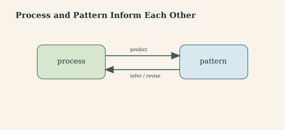
Biological modelling asks: which mechanisms could have produced the pattern we observe, and what patterns should follow if our mechanism is right?
\[\text{process}\Longleftrightarrow\text{pattern}.\]A model can run forward, from assumed processes (births, infection, competition) to predicted patterns (population cycles, epidemic curves, coexistence), or backward, from observed patterns to the processes that could explain them. Its value is not that it makes biology simple. Its value is that it makes assumptions explicit, so that they can be argued about, tested, and revised.
The notes start with the simplest possible model, a population that grows, and add one biological mechanism at a time. Each addition brings a new mathematical tool:
| Section | Biological mechanism | Mathematical tool |
|---|---|---|
| 1-2 | building a model | flow diagrams, units |
| 3 | reproduction | recursions, differential equations, exponential growth |
| 4 | density dependence | logistic growth, analytical solutions |
| 5 | - | phase lines, cobwebs, numerical solution in R |
| 6 | - | equilibria and local stability in one variable |
| 7 | harvesting | yield optimization, saddle-node bifurcation |
| 8 | competition, predation | phase planes, nullclines, Jacobians |
| 9 | infection | compartment models, $R_0$, final size |
| 10 | - | bifurcations and chaos |
| 11 | age structure | matrices, eigenvalues |
| 12 | natural selection | allele-frequency recursions |
| 13 | chance | birth-death processes, Gillespie simulation |
| 14 | data | fitting, identifiability, sensitivity |
1. Why Model?
1.1 Verbal Models Are Ambiguous
Consider the hypothesis “a predator controls its prey population”. Does it predict that prey numbers stay constant? That they cycle? That adding more predators lowers prey numbers permanently, or only temporarily? A verbal statement cannot answer these questions, because it does not say how much predators eat, how this depends on prey density, or how fast predators reproduce. Writing the hypothesis as an equation forces those decisions. Often, the act of writing the model reveals that two people who “agree” on a verbal hypothesis meant different things.
1.2 Kinds of Models
| Choice | Option A | Option B |
|---|---|---|
| Purpose | phenomenological (describes a pattern, e.g. a curve fit) | mechanistic (derives the pattern from processes) |
| Time | discrete (generations, years) | continuous (rates) |
| Randomness | deterministic (average behaviour) | stochastic (chance events) |
| Structure | unstructured (one number per population) | structured (age, space, genotype, individual) |
There is no best choice in general. The biology and the question decide. A useful attitude is the famous one: all models are wrong, some are useful. A model is useful when it is simple enough to understand and rich enough to contain the mechanism you care about.
2. Building a Model Step by Step
Otto and Day give a recipe that works for almost every model in this course.
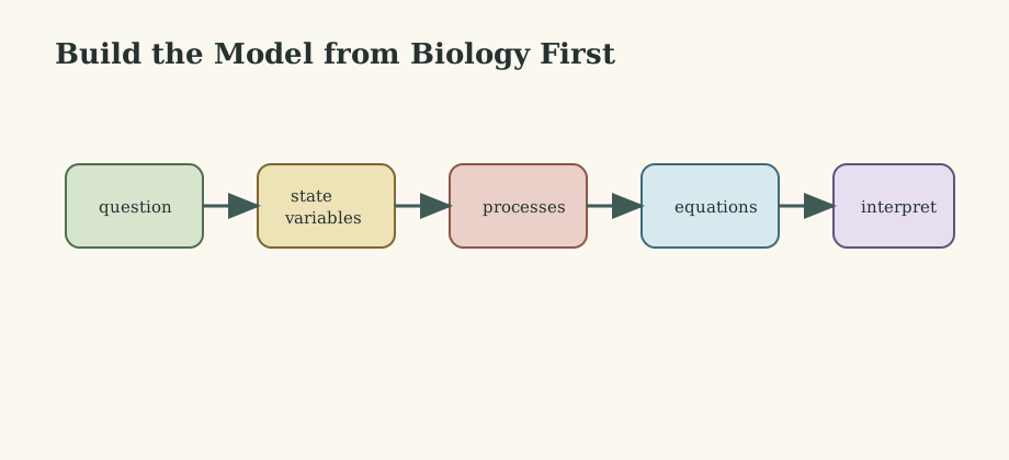
- Formulate the question. “Will this fish stock persist under the current fishing pressure?”
- Choose the state variables: the quantities that change. Here, $N(t)$, the number of fish.
- List the processes that change them: births, natural deaths, harvest.
- Draw a flow diagram: a box for $N$, an arrow in for births, arrows out for deaths and harvest, each labelled with its rate.
- Translate to equations: rate of change = inflows - outflows.
- Analyse: equilibria, stability, numerical solutions, parameter dependence.
- Check and interpret: units, limiting cases, comparison with data; return to step 1 if needed.
Worked translation. Suppose each fish produces offspring at per-capita rate $\beta$ (per year), dies naturally at per-capita rate $\mu$, and is caught at per-capita rate $E$ (fishing effort). Then
\[\frac{dN}{dt}=\underbrace{\beta N}_{\text{births}}-\underbrace{\mu N}_{\text{deaths}}-\underbrace{EN}_{\text{harvest}}=(\beta-\mu-E)\,N.\]Check the units. $dN/dt$ has units of fish per year. Each term on the right must too: $\beta$ is per year and $N$ is fish, so $\beta N$ is fish per year. A unit mismatch is the fastest way to catch a modelling error.
Check limiting cases. With no fishing and $\beta=\mu$, the population is constant. With $E$ very large, the population declines. If a model fails such sanity checks, find out why before doing anything else.
3. Discrete and Continuous Growth
3.1 Geometric Growth in Discrete Time
For organisms that reproduce once a year (annual plants, many insects), write the population at the next census as a function of the current one, a recursion:
\[N(t+1)=\lambda\,N(t),\]where $\lambda$ is the finite rate of increase: the average number of individuals next year per individual this year (surviving adults plus offspring). Iterating,
\[N(t)=\lambda^tN(0).\]The population grows if $\lambda>1$, declines if $\lambda < 1$.
3.2 Exponential Growth in Continuous Time
For organisms with overlapping generations and births throughout the year, use rates. If $r$ is the per-capita growth rate (births minus deaths per individual per unit time),
\[\frac{dN}{dt}=rN\qquad\Longrightarrow\qquad N(t)=N(0)\,e^{rt}.\]The two descriptions match when $\lambda=e^r$, i.e. $r=\ln\lambda$: growth if $r>0$, decline if $r < 0$.
A handy quantity is the doubling time, from $e^{rT_2}=2$:
\[T_2=\frac{\ln2}{r}.\]With $r=0.1$ per year, the population doubles every $6.9$ years.
3.3 Which to Choose?
Discrete time suits seasonal reproduction, annual census data, and non-overlapping generations. Continuous time suits overlapping generations, physiology, infection, and movement. The two can behave very differently once density dependence is added (section 6.4): discrete-time models can overshoot, because the population “decides” next year’s size based on this year’s density, a built-in time delay.
What to Remember
- Discrete: $N(t+1)=\lambda N(t)$, $N(t)=\lambda^tN(0)$. Continuous: $dN/dt=rN$, $N(t)=N(0)e^{rt}$.
- $r=\ln\lambda$; doubling time $\ln2/r$.
- Exponential growth is a good local description and an impossible long-run one.
4. Density Dependence: The Logistic Model
4.1 From Assumption to Equation
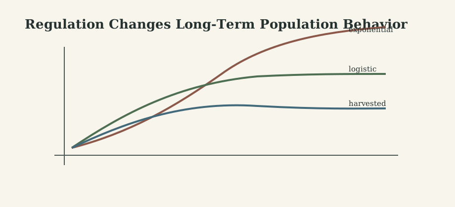
No population grows exponentially forever; resources run out. The simplest assumption is that the per-capita growth rate declines linearly with density, from $r$ when the population is tiny to zero at the carrying capacity $K$:
\[\frac1N\frac{dN}{dt}=r\Big(1-\frac NK\Big)\qquad\Longrightarrow\qquad\frac{dN}{dt}=rN\Big(1-\frac NK\Big).\]The model has two equilibria, $N=0$ and $N=K$. The population growth rate $rN(1-N/K)$ is a parabola in $N$ with its maximum at $N=K/2$, where it equals $rK/4$. This number reappears in harvesting (section 7).
4.2 The Analytical Solution
The logistic equation is separable. Using partial fractions,
\[\int\frac{dN}{N(1-N/K)}=\int r\,dt\quad\Longrightarrow\quad N(t)=\frac{K}{1+\Big(\dfrac{K-N(0)}{N(0)}\Big)e^{-rt}}.\]The solution is the familiar S-shaped curve: nearly exponential at first, an inflection point at $N=K/2$, then saturation at $K$. Having an explicit solution is rare; most models in these notes do not have one, which is why sections 5 and 6 matter.
4.3 Discrete-Time Versions
Several recursions express density dependence in discrete time:
\[\begin{aligned} &\text{discrete logistic:} && N(t+1)=N(t)+rN(t)\Big(1-\frac{N(t)}K\Big),\\ &\text{Beverton-Holt:} && N(t+1)=\frac{\lambda N(t)}{1+(\lambda-1)N(t)/K},\\ &\text{Ricker:} && N(t+1)=N(t)\,e^{r(1-N(t)/K)}. \end{aligned}\]They have the same equilibria ($0$ and $K$) but different shapes, and, as section 6.4 shows, very different dynamics. Beverton-Holt always approaches $K$ smoothly (it models contest competition, where some individuals always get enough); the discrete logistic and the Ricker model can oscillate and even become chaotic (scramble competition, where everyone gets too little at high density).
What to Remember
- Logistic: per-capita growth declines linearly with $N$; equilibria $0$ and $K$; maximum growth $rK/4$ at $N=K/2$.
- Explicit S-shaped solution in continuous time.
- Discrete versions share equilibria but can behave very differently.
5. Graphical and Numerical Analysis
5.1 The Phase Line
For a one-variable continuous model $dN/dt=f(N)$, plot $f(N)$ against $N$. Where $f>0$, $N$ increases (arrow to the right); where $f < 0$, it decreases (arrow to the left); where $f=0$, there is an equilibrium. For the logistic model, $f$ is an upside-down parabola: arrows point away from $0$ and towards $K$. You can read off the long-term behaviour from every starting point without solving anything.
5.2 Cobweb Diagrams for Recursions
For $N(t+1)=F(N(t))$, plot $F(N)$ together with the diagonal $N(t+1)=N(t)$. Start at $N(0)$ on the horizontal axis, go up to the curve to find $N(1)$, across to the diagonal to move $N(1)$ back onto the horizontal axis, up to the curve again, and so on. Equilibria are where the curve crosses the diagonal. The cobweb shows monotone approach, damped oscillation, cycles, or chaos at a glance.
5.3 Numerical Solution: Euler’s Method
Most models have no explicit solution, so we compute approximate trajectories. The simplest method follows the slope for a short step $\Delta t$:
\[N(t+\Delta t)\approx N(t)+\Delta t\,f\big(N(t)\big).\]How accurate is it? Take $dN/dt=N$, $N(0)=1$, whose exact value at $t=1$ is $e\approx2.718$. With $\Delta t=0.1$, ten Euler steps give $1.1^{10}=2.594$, a 4.6% error. With $\Delta t=0.01$, a hundred steps give $1.01^{100}=2.705$, a 0.5% error. Ten times smaller steps, ten times smaller error: Euler’s method is first-order accurate. Note also that Euler with a large step turns a continuous model into a discrete one, which can oscillate spuriously; a numerical artefact can look like biology.
In practice, use a higher-order adaptive solver. In R, deSolve::ode (default method lsoda) chooses step sizes automatically:
library(deSolve)

logistic <- function(t, state, parms) {
  with(as.list(c(state, parms)), {
    dN <- r * N * (1 - N / K)
    list(c(dN))
  })
}

out <- ode(y = c(N = 10), times = seq(0, 50, by = 0.1),
           func = logistic, parms = c(r = 0.3, K = 1000))
plot(out, xlab = "time", ylab = "N", main = "Logistic growth")
Recursions need no solver, just a loop:
ricker <- function(N0, r, K, steps) {
  N <- numeric(steps + 1)
  N[1] <- N0
  for (t in 1:steps) N[t + 1] <- N[t] * exp(r * (1 - N[t] / K))
  N
}
plot(0:50, ricker(10, 1.8, 1000, 50), type = "b", xlab = "year", ylab = "N")
What to Remember
- Phase lines (continuous) and cobwebs (discrete) show qualitative dynamics without solving.
- Euler is first-order: error proportional to $\Delta t$. Use adaptive solvers (
deSolve::ode). - Check that numerical behaviour does not depend on the step size.
6. Equilibria and Stability in One Variable
6.1 Finding Equilibria
An equilibrium $\hat N$ satisfies $dN/dt=0$ (continuous) or $N(t+1)=N(t)$ (discrete). For the logistic model, $rN(1-N/K)=0$ gives $\hat N=0$ and $\hat N=K$.
6.2 Local Stability, Continuous Time
Is the equilibrium an attractor? Perturb it: $N=\hat N+\varepsilon$. Taylor expansion of $f$ around $\hat N$, using $f(\hat N)=0$, gives
\[\frac{d\varepsilon}{dt}\approx f'(\hat N)\,\varepsilon\qquad\Longrightarrow\qquad\varepsilon(t)\approx\varepsilon(0)\,e^{f'(\hat N)t}.\]So $\hat N$ is locally stable if \(f'(\hat N) < 0\) and unstable if \(f'(\hat N)>0\). The magnitude of \(f'(\hat N)\) is the rate of return, and \(1/\lvert f'(\hat N)\rvert\) is the characteristic return time.
Logistic. $f(N)=rN-rN^2/K$, so \(f'(N)=r-2rN/K\). At $\hat N=0$: \(f'=r>0\), unstable (a small population grows). At $\hat N=K$: \(f'=-r < 0\), stable, with return time $1/r$.
6.3 Local Stability, Discrete Time
For $N(t+1)=F(N(t))$, a perturbation obeys \(\varepsilon(t+1)\approx F'(\hat N)\,\varepsilon(t)\), so \(\varepsilon(t)\approx F'(\hat N)^t\varepsilon(0)\). The equilibrium is locally stable if \(\lvert F'(\hat N)\rvert < 1\). The sign matters too:
| \(F'(\hat N)\) | Behaviour near $\hat N$ |
|---|---|
| \(0 < F' < 1\) | monotone approach |
| \(-1 < F' < 0\) | damped oscillation |
| \(F' < -1\) | growing oscillation (unstable) |
| \(F'>1\) | monotone departure (unstable) |
6.4 Worked Example: The Discrete Logistic Can Oscillate
For $F(N)=N+rN(1-N/K)$, we get \(F'(N)=1+r-2rN/K\), so \(F'(K)=1-r\). Hence:
- $0 < r < 1$: \(F'(K)\in(0,1)\), smooth approach to $K$;
- $1 < r < 2$: \(F'(K)\in(-1,0)\), damped oscillations around $K$;
- $r>2$: \(\lvert F'(K)\rvert>1\), the equilibrium is unstable.
What happens beyond $r=2$? Iterating numerically, the population settles on a 2-cycle (alternating high and low years) for $2 < r < 2.449$, a 4-cycle up to about $2.544$, then 8, 16, … cycles in ever-shorter intervals, and chaos beyond about $r\approx2.57$: deterministic but aperiodic, and sensitive to initial conditions. The Ricker model has the same stability condition, \(F'(K)=1-r\), and the same route to chaos. Robert May’s 1976 paper on this simple equation changed how ecologists think about population fluctuations: irregular dynamics do not require random environments.
The continuous logistic equation can never do this; in one dimension, a continuous trajectory cannot overshoot an equilibrium. The difference is the built-in delay of the discrete model.
What to Remember
- Continuous: stable if \(f'(\hat N) < 0\). Discrete: stable if \(\lvert F'(\hat N)\rvert < 1\); negative slope means oscillation.
- The discrete logistic is stable for $0 < r < 2$, then period-doubles to chaos.
- Delays (discrete generations) can destabilize; continuous one-variable models cannot oscillate.
7. Harvesting: Yield, Stability, and Collapse
7.1 Constant Effort
Harvest a logistic population in proportion to its size (constant fishing effort $E$). With the course’s parameterization $r$, $\alpha=r/K$:
\[\frac{dN}{dt}=N(r-\alpha N)-EN.\]The nonzero equilibrium is $\hat N=\frac{r-E}{\alpha}=K\big(1-\frac Er\big)$, which exists if $E < r$. Its stability: \(f'(\hat N)=r-E-2\alpha\hat N=-(r-E) < 0\). Stable. The sustainable yield at equilibrium is
\[Y(E)=E\hat N=\frac{E(r-E)}{\alpha},\]maximized at $E=r/2$, giving the maximum sustainable yield $\mathrm{MSY}=\frac{r^2}{4\alpha}=\frac{rK}{4}$, with the stock at $K/2$. Note that the return rate to equilibrium, $r-E$, is halved at MSY: the harvested stock recovers from disturbances more slowly.
7.2 Constant Quota and a Tipping Point
Now harvest a fixed amount $H$ per year regardless of stock size:
\[\frac{dN}{dt}=rN\Big(1-\frac NK\Big)-H.\]Equilibria are where the parabola $rN(1-N/K)$ meets the horizontal line $H$.
Worked example. $r=0.5$ per year, $K=1000$, so $\mathrm{MSY}=125$. With quota $H=100$:
\[0.5N\Big(1-\frac N{1000}\Big)=100\iff N^2-1000N+200{,}000=0\iff N=723.6\ \text{or}\ 276.4.\]From the phase line: the upper equilibrium (723.6) is stable; the lower one (276.4) is unstable, a threshold. A stock pushed below 276.4 (by a bad year or a survey error) declines to extinction even though the quota has not changed.
As $H$ increases towards 125, the two equilibria approach each other; at $H=rK/4$ they merge and disappear. For $H>125$ there is no equilibrium and the stock collapses from any starting size. This is a saddle-node bifurcation: a small change in a parameter produces a sudden, qualitative change, and reducing $H$ slightly afterwards does not bring the stock back. Constant quotas are inherently riskier than constant effort, and setting a quota at the estimated MSY leaves no margin for error.
What to Remember
- Constant effort: stable equilibrium, MSY $=rK/4$ at $N=K/2$ and $E=r/2$.
- Constant quota: two equilibria (stable and threshold) that collide at $H=rK/4$; beyond it, collapse.
- Bifurcations turn small parameter changes into qualitative shifts.
8. Two Interacting Species
8.1 Tools for Two Variables
For $\dot x=f(x,y)$, $\dot y=g(x,y)$:
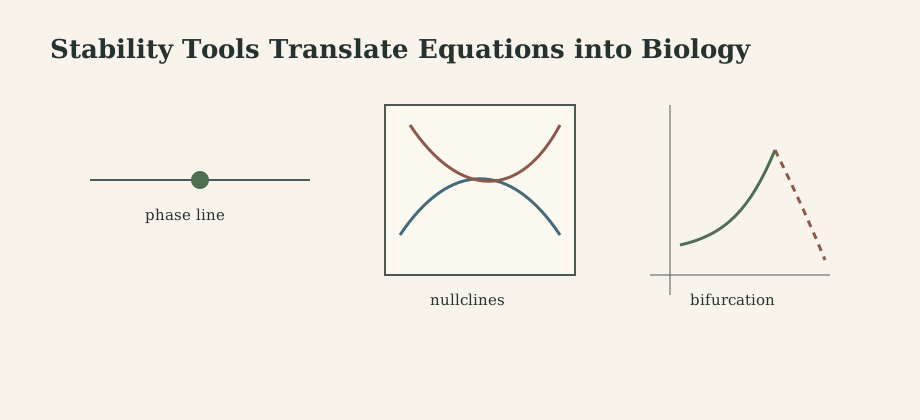
- Nullclines: the curves where $\dot x=0$ and where $\dot y=0$. Equilibria are their intersections. Between nullclines, the direction of motion is known from the signs of $f$ and $g$.
- Jacobian: near an equilibrium, perturbations obey $\dot{\varepsilon}=J\varepsilon$ with
The equilibrium is locally stable if both eigenvalues have negative real parts. For $2\times2$ matrices this is equivalent to
\[\mathrm{tr}\,J<0\quad\text{and}\quad\det J>0.\]The trace-determinant plane classifies the rest: $\det J < 0$ gives a saddle; $\mathrm{tr}^2 < 4\det$ gives complex eigenvalues (spirals); $\mathrm{tr}=0$ with $\det>0$ gives a center.
8.2 Lotka-Volterra Competition
Two species share resources; each reduces the other’s growth:
\[\frac{dN_1}{dt}=r_1N_1\Big(1-\frac{N_1+\alpha_{12}N_2}{K_1}\Big),\qquad \frac{dN_2}{dt}=r_2N_2\Big(1-\frac{N_2+\alpha_{21}N_1}{K_2}\Big).\]The competition coefficient $\alpha_{12}$ converts individuals of species 2 into “equivalents” of species 1. The nonzero nullclines are straight lines: $N_1+\alpha_{12}N_2=K_1$ and $N_2+\alpha_{21}N_1=K_2$. Their arrangement gives four outcomes:
| Condition | Outcome |
|---|---|
| $\alpha_{12} < K_1/K_2$ and $\alpha_{21} < K_2/K_1$ | stable coexistence |
| $\alpha_{12}>K_1/K_2$ and $\alpha_{21}>K_2/K_1$ | bistability: whoever starts ahead wins |
| $\alpha_{12} < K_1/K_2$ and $\alpha_{21}>K_2/K_1$ | species 1 wins |
| $\alpha_{12}>K_1/K_2$ and $\alpha_{21} < K_2/K_1$ | species 2 wins |
With equal carrying capacities, coexistence requires $\alpha_{12} < 1$ and $\alpha_{21} < 1$: each species must limit itself more than it limits the other. This is the mathematical form of the competitive exclusion principle and of niche differentiation.
8.3 Lotka-Volterra Predator-Prey
Prey $R$ grow exponentially and are eaten at a rate proportional to encounters; predators convert food into offspring with efficiency $c$ and die at rate $d$:
\[\frac{dR}{dt}=bR-aRP,\qquad\frac{dP}{dt}=caRP-dP.\]The coexistence equilibrium is $\hat R=\frac{d}{ca}$, $\hat P=\frac ba$. Note the surprise: the prey equilibrium depends only on predator parameters, and vice versa. The Jacobian there is
\[J=\begin{bmatrix}0&-d/c\\cb&0\end{bmatrix},\qquad\mathrm{tr}\,J=0,\quad\det J=bd>0,\]so the eigenvalues are $\pm i\sqrt{bd}$: a center. Trajectories are closed cycles, with period about $2\pi/\sqrt{bd}$ near the equilibrium, and predator peaks lagging prey peaks by a quarter cycle. But the amplitude depends entirely on the initial condition, and any small change to the model (density dependence, saturation) destroys the neutral cycles. The model is structurally unstable: a good starting point, not a final answer.
8.4 Functional Responses: How Much Does a Predator Eat?
The term $aRP$ assumes that each predator eats prey at a rate proportional to prey density, forever: a type I functional response. Real predators spend time handling prey. Derive the alternative from a time budget: in total time $T$, a predator searches for time $T_s$ and handles each captured prey for time $h$. Captures are $C=aRT_s$ and $T=T_s+hC$. Solving,
\[\frac CT=F(R)=\frac{aR}{1+ahR},\]the Holling type II response, with search efficiency $a$ and handling time $h$. At low density it is approximately $aR$; at high density it saturates at $1/h$, the maximum rate set by handling. A type III response, $F(R)=\frac{aR^2}{1+ahR^2}$, is sigmoid, as when predators switch to other prey or prey have refuges at low density.
These shapes are not cosmetic. A saturating response weakens predation at high prey density, which tends to destabilize; a sigmoid one strengthens it at low density relative to linear, which tends to stabilize. Interaction terms should be chosen from biology, not for algebraic convenience.
8.5 The Paradox of Enrichment
Combine logistic prey with a type II predator (the Rosenzweig-MacArthur model):
\[\frac{dR}{dt}=rR\Big(1-\frac RK\Big)-\frac{aRP}{1+ahR},\qquad \frac{dP}{dt}=\frac{eaRP}{1+ahR}-mP.\]The predator nullcline is a vertical line $R=\hat R=\frac{m}{a(e-mh)}$. The prey nullcline, $P=\frac ra\big(1-\frac RK\big)(1+ahR)$, is a hump with its peak at $R=\frac12\big(K-\frac1{ah}\big)$. The equilibrium is stable when the predator nullcline crosses to the right of the hump, and unstable, surrounded by a stable limit cycle, when it crosses to the left.
Now enrich the system by raising $K$ (more nutrients). The hump moves right, past $\hat R$, and the equilibrium loses stability through a Hopf bifurcation: populations begin to cycle with growing amplitude, and at low points of the cycle may go extinct. Rosenzweig called this the paradox of enrichment: more food can destabilize a food chain.
What to Remember
- Two variables: nullclines, then the Jacobian; stable iff $\mathrm{tr}\,J < 0$ and $\det J>0$.
- Competition: coexistence when intraspecific limits exceed interspecific ones.
- LV predator-prey gives neutral cycles (structurally unstable); handling time gives type II responses.
- Enrichment can destabilize predator-prey systems (Hopf bifurcation).
9. Epidemics: Compartment Models
9.1 The SIR Model
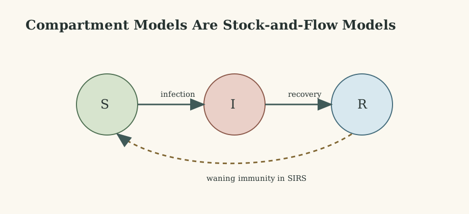
Divide a population of size $N$ into susceptible $S$, infectious $I$, and recovered $R$. Contacts between susceptible and infectious individuals cause infections at rate $\frac bNSI$ (each infectious person makes $b$ infecting contacts per day if everyone is susceptible), and infectious individuals recover after an average time $T_r$:
\[\frac{dS}{dt}=-\frac bNSI,\qquad \frac{dI}{dt}=\frac bNSI-\frac I{T_r},\qquad \frac{dR}{dt}=\frac I{T_r}.\]The three equations sum to zero: $N$ is constant.
9.2 The Threshold and the Basic Reproduction Number
Early in an outbreak, $S\approx N$, so $\frac{dI}{dt}\approx\big(b-\frac1{T_r}\big)I$. Infections grow if
\[b-\frac1{T_r}>0\iff R_0=bT_r>1.\]The basic reproduction number $R_0$ is the expected number of secondary infections caused by one infectious individual in a fully susceptible population: infecting contacts per day times days infectious.
Worked numbers. With $b=0.5$ per day and $T_r=4$ days, $R_0=2$. The early growth rate is $b-1/T_r=0.25$ per day, so cases double every $\ln2/0.25\approx2.8$ days.
More generally, $\frac{dI}{dt}>0$ whenever $S>N/R_0$. So the epidemic peaks when the susceptible fraction falls to $1/R_0$: in the example, when half the population is still susceptible. Simulating with $N=1000$ and one initial case, the peak comes around day 27 with about 154 people infectious at once.
9.3 How Many Get Infected? The Final Size
Divide the $S$ and $R$ equations: $\frac{dS}{dR}=-\frac{R_0}{N}S$, so $S=S(0)\,e^{-R_0R/N}$. At the end of the epidemic $I=0$, so $R(\infty)=N-S(\infty)$. With $S(0)\approx N$ and writing $s_\infty=S(\infty)/N$:
\[s_\infty=e^{-R_0(1-s_\infty)}.\]For $R_0=2$, solving numerically gives $s_\infty\approx0.203$: about 80% of the population is eventually infected. Note that this is much more than the 50% needed to stop growth: the epidemic overshoots the herd-immunity threshold, because infections continue after the peak while many people are still infectious.
9.4 Vaccination and Herd Immunity
If a fraction $p$ is immune before the outbreak, the effective reproduction number is $R_0(1-p)$, and the outbreak cannot grow if
\[p>p_c=1-\frac1{R_0}.\]For $R_0=2$, $p_c=50\%$; for measles, with $R_0$ often quoted around 12-18, over 90%.
9.5 SIRS: Waning Immunity and Endemic Infection
If immunity lasts an average time $T_i$, recovered individuals return to the susceptible pool:
\[\frac{dS}{dt}=-\frac bNSI+\frac R{T_i},\qquad \frac{dI}{dt}=\frac bNSI-\frac I{T_r},\qquad \frac{dR}{dt}=\frac I{T_r}-\frac R{T_i}.\]Now the infection can persist. At an endemic equilibrium, $\frac{dI}{dt}=0$ requires $\hat S=N/R_0$, and $\frac{dR}{dt}=0$ gives $\hat R=\frac{T_i}{T_r}\hat I$. Using $\hat S+\hat I+\hat R=N$:
\[\hat I=N\Big(1-\frac1{R_0}\Big)\frac{T_r}{T_r+T_i}.\]It exists (is positive) exactly when $R_0>1$. As $R_0$ crosses 1, the disease-free equilibrium loses stability and the endemic one appears: a transcritical bifurcation. Approach to the endemic state is typically through damped oscillations, so recurrent waves can appear even in this deterministic model. Adding births and deaths at rate $\mu$ has a similar effect, with $R_0=\frac{b}{1/T_r+\mu}$.
9.6 Solving SIR in R
library(deSolve)

sir <- function(t, y, p) {
  with(as.list(c(y, p)), {
    N  <- S + I + R
    dS <- -b / N * S * I
    dI <-  b / N * S * I - I / Tr
    dR <-  I / Tr
    list(c(dS, dI, dR))
  })
}

out <- ode(y = c(S = 999, I = 1, R = 0), times = seq(0, 100, by = 0.5),
           func = sir, parms = c(b = 0.5, Tr = 4))
matplot(out[, "time"], out[, c("S", "I", "R")], type = "l", lty = 1,
        xlab = "day", ylab = "individuals")
legend("right", c("S", "I", "R"), col = 1:3, lty = 1)
What to Remember
- SIR: $R_0=bT_r$; growth iff $R_0>1$; peak when $S/N=1/R_0$.
- Final size: $s_\infty=e^{-R_0(1-s_\infty)}$ (about 80% infected for $R_0=2$): overshoot beyond herd immunity.
- Vaccination threshold $1-1/R_0$. SIRS allows endemic equilibrium $\hat I=N(1-1/R_0)T_r/(T_r+T_i)$.
10. Bifurcations: When Parameters Change Behaviour
A bifurcation is a parameter value at which the qualitative behaviour of a model changes: equilibria appear, disappear, or change stability, or cycles are born. We have now met the main types:
| Bifurcation | What happens | Example in these notes |
|---|---|---|
| Saddle-node | two equilibria collide and vanish | quota harvesting at $H=rK/4$ |
| Transcritical | two equilibria cross and exchange stability | SIRS at $R_0=1$ |
| Pitchfork | one equilibrium splits into three (symmetric systems) | symmetric competition, some selection models |
| Hopf | a stable equilibrium becomes unstable, a limit cycle appears | Rosenzweig-MacArthur under enrichment |
| Period-doubling | a cycle of period $k$ becomes period $2k$ | discrete logistic at $r=2$, $2.449$, … |
A bifurcation diagram plots the long-term states (equilibria or the values visited by a cycle) against a parameter. For the discrete logistic, it shows the cascade of period doublings into chaos:
r_values <- seq(1.5, 3, by = 0.002)
plot(NULL, xlim = range(r_values), ylim = c(0, 1.4),
     xlab = "r", ylab = "N / K")
for (r in r_values) {
  x <- 0.5
  for (i in 1:500) x <- x + r * x * (1 - x)        # discard the transient
  xs <- numeric(100)
  for (i in 1:100) { x <- x + r * x * (1 - x); xs[i] <- x }
  points(rep(r, 100), xs, pch = ".")
}
Bifurcations matter in management because they mark tipping points: near a saddle-node or Hopf bifurcation, recovery from disturbances slows down (“critical slowing down”), which is one proposed early-warning signal of impending collapse.
11. Structured Populations and Matrices
11.1 Leslie Matrices
Individuals of different ages survive and reproduce differently. Divide a population into age classes and track the vector $n(t)$. With fecundities $F_i$ and survival probabilities $s_i$ from class $i$ to $i+1$, the Leslie matrix model is $n(t+1)=L\,n(t)$. For three age classes:
\[L=\begin{bmatrix}F_1&F_2&F_3\\s_1&0&0\\0&s_2&0\end{bmatrix}=\begin{bmatrix}0&1.5&1.0\\0.5&0&0\\0&0.8&0\end{bmatrix}.\]11.2 Eigenvalues Give the Long-Run Behaviour
Iterating, $n(t)=L^tn(0)$. Expand $n(0)$ in eigenvectors of $L$: each component grows like $\lambda_i^t$, so in the long run the dominant eigenvalue $\lambda_1$ takes over:
- $\lambda_1$ is the long-run growth rate per time step (the structured version of section 3.1);
- its eigenvector is the stable age distribution, the proportions the population converges to regardless of its starting composition.
For the example, the characteristic polynomial is $\lambda^3-0.75\lambda-0.4=0$, with dominant root $\lambda_1\approx1.062$: the population grows about 6% per time step. The stable age distribution is about $(0.55,\ 0.26,\ 0.19)$: 55% newborns, 26% one-year-olds, 19% two-year-olds.
Sensitivity analysis asks which entry of $L$ most affects $\lambda_1$. For long-lived species (turtles, large mammals), adult survival often matters far more than fecundity, which tells conservation managers where effort pays off.
What to Remember
- Age-structured dynamics: $n(t+1)=Ln(t)$.
- Dominant eigenvalue = long-run growth rate; its eigenvector = stable age distribution.
- Sensitivities of $\lambda_1$ guide management.
12. Natural Selection
12.1 Haploid Selection
Consider two alleles, $A$ (frequency $p$) and $a$ (frequency $1-p$), in a haploid population with fitnesses $W_A$ and $W_a$ (expected offspring per individual). After one generation of selection, each type is represented in proportion to its frequency times its fitness:
\[p(t+1)=\frac{p(t)\,W_A}{p(t)\,W_A+\big(1-p(t)\big)W_a}=\frac{p(t)\,W_A}{\bar W}.\]The denominator $\bar W$ is the mean fitness. The equilibria are $p=0$ and $p=1$; if $W_A>W_a$, $p=1$ is stable and $A$ goes to fixation.
How fast? The odds ratio is simple: $\frac{p(t)}{1-p(t)}=\Big(\frac{W_A}{W_a}\Big)^t\frac{p(0)}{1-p(0)}$. With a 1% fitness advantage ($W_A/W_a=1.01$), going from a frequency of $1\%$ to $99\%$ multiplies the odds by $99^2\approx9800$, which takes $\ln9800/\ln1.01\approx920$ generations. Selection is powerful but not instantaneous.
12.2 Diploids and Frequency Dependence
In diploids, fitness depends on the genotype ($AA$, $Aa$, $aa$), and dominance matters: a recessive beneficial allele spreads very slowly at first because it is almost never in the homozygous form. Heterozygote advantage maintains both alleles at a stable internal equilibrium (the classic example is the sickle-cell allele in malaria regions). When fitness depends on the frequencies of other types, we are in evolutionary game theory: the Hawk-Dove game, with its stable mixture of $V/C$ hawks, is a selection model (see the game theory note).
What to Remember
- Haploid selection: \(p'=pW_A/\bar W\); the odds change by the factor $W_A/W_a$ per generation.
- Small fitness differences need hundreds to thousands of generations.
- Dominance, heterozygote advantage, and frequency dependence change the outcome.
13. Stochastic Models
13.1 Why Chance Matters
Deterministic models describe average behaviour. Real populations are made of individuals who are born and die at random times. In large populations, this demographic stochasticity averages out; in small populations, it can drive extinction even when the average growth rate is positive. Environments also fluctuate (environmental stochasticity), affecting everyone at once. Both matter in conservation, invasion biology, and epidemics.
13.2 Birth-Death Processes and Extinction
In the simplest stochastic model, each individual gives birth at rate $b$ and dies at rate $d$. The deterministic version is $dN/dt=(b-d)N$, exponential growth if $b>d$. In the stochastic version, the population can still hit zero by a run of bad luck. The probability of eventual extinction starting from $N_0$ individuals is
\[P_{\text{ext}}=\begin{cases}(d/b)^{N_0},&b>d,\\1,&b\le d.\end{cases}\]Worked numbers. With $b=1.2$ and $d=1.0$ (a growing population on average), a single founder goes extinct with probability $1/1.2\approx0.83$; ten founders with probability $0.83^{10}\approx0.16$. Simulations reproduce both numbers. Most introductions of a few individuals fail even when conditions are favourable, which matters for invasions, reintroductions, and new mutations.
13.3 The Gillespie Algorithm
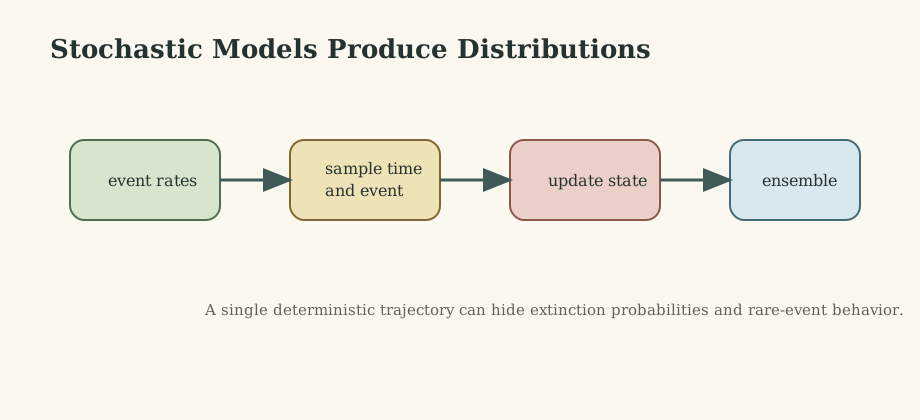
To simulate a continuous-time stochastic model exactly, list the possible events and their rates. For SIR: infection at rate $bSI/N$ and recovery at rate $I/T_r$. Then repeat:
- compute the total rate $\Lambda$ of all events;
- draw the time to the next event from an exponential distribution with rate $\Lambda$;
- choose which event happens, with probability proportional to its rate;
- update the state and the clock.
gillespie_sir <- function(S, I, R, b, Tr, t_max) {
  N <- S + I + R
  t <- 0
  out <- data.frame(t = t, S = S, I = I, R = R)
  while (t < t_max && I > 0) {
    rate_inf <- b * S * I / N
    rate_rec <- I / Tr
    total    <- rate_inf + rate_rec
    t <- t + rexp(1, total)                 # time to the next event
    if (runif(1) < rate_inf / total) {      # which event?
      S <- S - 1; I <- I + 1
    } else {
      I <- I - 1; R <- R + 1
    }
    out[nrow(out) + 1, ] <- c(t, S, I, R)
  }
  out
}

set.seed(1)
runs <- replicate(200, tail(gillespie_sir(999, 1, 0, 0.5, 4, 365)$R, 1))
hist(runs, breaks = 40, xlab = "final number recovered", main = "")
Run many times, this reveals what the deterministic model hides. With $R_0=2$ and one initial case, about half of the simulated epidemics fizzle out after a handful of cases, while the rest grow into major outbreaks infecting about 80% of the population. The theory agrees: for one initial case, the probability of a major outbreak is approximately $1-1/R_0$. The histogram of final sizes is bimodal, something no single deterministic trajectory can show.
13.4 Environmental Stochasticity: The Geometric Mean
Suppose a population’s growth factor is $\lambda=1.5$ in good years and $\lambda=0.6$ in bad years, each with probability $\frac12$. The average growth factor is $1.05$, suggesting growth. But over many years, the population is multiplied by a product of factors, and
\[N(t)\approx N(0)\,\big(\lambda_{\text{good}}\lambda_{\text{bad}}\big)^{t/2}=N(0)\,(0.9)^{t/2},\]so the long-run growth factor per year is the geometric mean $\sqrt{1.5\times0.6}\approx0.949 < 1$: the population declines. Variability reduces long-run growth, which is why bet-hedging strategies (seed dormancy, spreading reproduction across years) can be favoured even if they lower average fitness.
What to Remember
- Demographic stochasticity can extinguish growing populations: $P_{\text{ext}}=(d/b)^{N_0}$.
- Gillespie simulation is exact for event-based models; run many replicates and look at distributions.
- One case with $R_0=2$: about 50% chance of a major outbreak. Environmental variability lowers long-run growth (geometric mean).
14. Connecting Models to Data
A model becomes science when it meets data.
- Fitting. Choose parameters to minimize the mismatch between model output and observations, by least squares or, better, by maximizing a likelihood that reflects how the data were collected (e.g. Poisson-distributed case counts). In R,
optimcombined withodedoes this for small models. - Identifiability. Some parameters cannot be separated by the data. In the early phase of an epidemic, case counts reveal the growth rate $b-1/T_r$, but not $b$ and $T_r$ separately; many combinations fit equally well. Check whether your data can actually determine what you want to estimate before trusting the estimates.
- Sensitivity analysis. Vary each parameter over its plausible range and see which ones change the conclusion. If the answer to the biological question flips within the uncertainty, say so.
- Model comparison. When several mechanisms fit, compare them with criteria that penalize complexity (AIC), and, more importantly, look for patterns where their predictions differ and collect data there.
- Out-of-sample checks. A model that fits past data may still fail to predict new conditions. Extrapolation beyond the observed regime is where models are most useful and most dangerous.
15. Workflow and Checklist
- Write the biological question in one sentence.
- Draw the flow diagram; list every assumption next to it.
- Write the equations; check units and limiting cases.
- Find equilibria; analyse their stability (derivative, Jacobian).
- Solve numerically (
deSolve::odefor ODEs, loops for recursions); confirm results do not depend on step size. - Sweep key parameters; look for bifurcations and thresholds.
- If numbers are small or variability matters, build the stochastic version and simulate replicates.
- Compare with data; check identifiability and sensitivity.
- Interpret biologically: which mechanism produced which pattern, and what would falsify it?
- Revise and repeat.
16. Summary
| Model | Equation | Key result |
|---|---|---|
| Geometric | $N(t+1)=\lambda N(t)$ | grows iff $\lambda>1$ |
| Exponential | $\dot N=rN$ | $N_0e^{rt}$; doubling time $\ln2/r$ |
| Logistic | $\dot N=rN(1-N/K)$ | $K$ stable; max growth $rK/4$ |
| Discrete logistic | \(N'=N+rN(1-N/K)\) | stable for $0 < r < 2$; period doubling to chaos |
| Harvest (effort) | $\dot N=N(r-\alpha N)-EN$ | MSY $=rK/4$ at $E=r/2$ |
| Harvest (quota) | $\dot N=rN(1-N/K)-H$ | saddle-node collapse at $H=rK/4$ |
| LV competition | linear nullclines | coexistence iff intra > inter limitation |
| LV predator-prey | $\dot R=bR-aRP$, $\dot P=caRP-dP$ | neutral cycles (center) |
| Holling II | $F(R)=aR/(1+ahR)$ | saturation at $1/h$; enrichment destabilizes |
| SIR | $R_0=bT_r$ | final size $s_\infty=e^{-R_0(1-s_\infty)}$; $p_c=1-1/R_0$ |
| SIRS | waning immunity $T_i$ | endemic $\hat I=N(1-1/R_0)T_r/(T_r+T_i)$ |
| Leslie | $n(t+1)=Ln(t)$ | growth rate = dominant eigenvalue |
| Haploid selection | \(p'=pW_A/\bar W\) | odds multiply by $W_A/W_a$ |
| Birth-death | rates $b$, $d$ | $P_{\text{ext}}=(d/b)^{N_0}$ |
Where models stop being reliable. A model can fit data while explaining little; parameters may be unmeasurable; mechanisms may be missing; extrapolation can fail outside the observed regime; and deterministic stability does not remove stochastic risk. The remedy is the loop at the top of these notes: state assumptions, derive predictions, confront data, and revise.
Where to go next: statistical inference for dynamic models (likelihood, Bayesian calibration), stochastic differential equations, spatial models and reaction-diffusion, individual-based models, adaptive dynamics, and network epidemiology.
References and Reading Guide
- S. P. Otto and T. Day, A Biologist’s Guide to Mathematical Modeling in Ecology and Evolution (Princeton, 2007). Chapters 2 (building models), 3 (classic models), 4 (numerical and graphical techniques), 5 (equilibria and stability in one variable), 7-8 (linear algebra, multivariable models), 10 (age structure), 13-14 (stochastic models). The main course text.
- J. D. Murray, Mathematical Biology I: An Introduction (3rd ed., Springer, 2002). Population dynamics, predator-prey, epidemics.
- M. J. Keeling and P. Rohani, Modeling Infectious Diseases in Humans and Animals (Princeton, 2008). SIR, SIRS, $R_0$, stochastic epidemics.
- N. J. Gotelli, A Primer of Ecology (4th ed., Sinauer, 2008). Gentle treatment of growth, competition, predation, and Leslie matrices.
- R. M. May, “Simple mathematical models with very complicated dynamics,” Nature 261, 1976.
- M. L. Rosenzweig, “Paradox of enrichment: destabilization of exploitation ecosystems in ecological time,” Science 171, 1971.
- D. T. Gillespie, “Exact stochastic simulation of coupled chemical reactions,” Journal of Physical Chemistry 81(25), 1977.
- H. Caswell, Matrix Population Models (2nd ed., Sinauer, 2001).
- K. Soetaert, T. Petzoldt, and R. W. Setzer, “Solving Differential Equations in R: Package deSolve,” Journal of Statistical Software 33(9), 2010.