Motor Control from Model to Hardware
Theory: Motors in the Loop: Actuators, Sensors, Models, Controllers and Sensor Fusion · KTH Royal Institute of Technology · September 2021 – March 2022
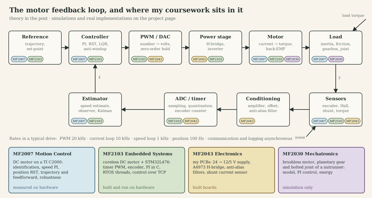
Goal: close a feedback loop around an electric motor and understand every link of it, from the control equation, through firmware, PWM, bridge and winding, to torque, and back through the encoder and the current sensor. The theory is in the companion post; this page is the engineering record: what was built, measured and simulated, what worked, and what turned out to be wrong.
Highlights
- Identified a DC motor from step and sine experiments ($J$, viscous and Coulomb friction) and closed speed, position and servo loops on a TI C2000. A directly designed discrete controller worked at a sampling period 25 times longer than its emulated counterpart.
- Wrote STM32 motor-control firmware (timer PWM, encoder interface, fixed-point PI) in three generations: super-loop, RTOS threads, and control split across two boards over TCP.
- Designed and built the electronics around the loop: a 24 V → 12/5 V supply, an A4973 H-bridge, anti-alias filters and a shunt current sensor.
- Designed two brushless drive shields for the Nucleo (DRV8323S, 60 V MOSFETs): a six-step velocity shield with Hall commutation and a field-oriented torque shield with three-shunt current sensing.
- Simulated an application drive, a brushless bolt-tightening tool, and found that the specified motor cannot meet both its torque and its speed requirement.
- Re-executed everything in Python, including the firmware with bit-exact C integer semantics. This exposed two unit errors in the simulation model and three overflow and actuation bugs in the firmware.
1. System architecture
The project used two hardware rigs, a set of custom boards and one simulation model, each covering different blocks of the loop:
| Platform | Hardware | Blocks of the loop | Kind |
|---|---|---|---|
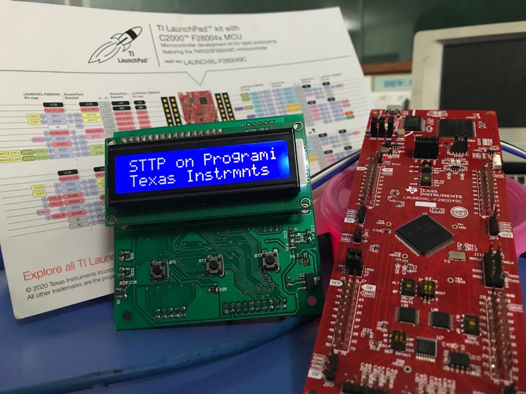
| Rig A: DC motor on C2000 | DC motor with 3600-pulse encoder, ±24 V amplifier, TI LAUNCHXL-F28379D, Simulink external mode | model identification, speed / position / servo control, sampling and anti-windup | real hardware |
| Rig B: STM32 speed controller | Nucleo-L476RG, dual half-bridge motor shield, Assun coreless DC motor with encoder, WIZnet W5500 Ethernet | PWM generation, encoder interface, embedded PI, RTOS, distributed control | real hardware |
| Custom boards | my PCBs, designed in Eagle | power supply, H-bridge with current chopper, anti-alias filters, current sensor | built |
| BLDC shields | Nucleo shields with DRV8323S, BSC028N06NS bridge, 5 mΩ shunts, Hall and encoder inputs | three-phase power stage, current sensing, Hall/encoder interface for velocity and torque control | designed (schematic + PCB) |
| Application model | MATLAB/Simulink | brushless motor + planetary gearbox + bolted joint of an Atlas Copco nutrunner | simulation |
</div>
2. Modelling and identification
2.1 Identifying the DC motor (Rig A)
Step responses at 7, 12 and 18 V and sine inputs at 0.5 rad/s were fitted to the DC-motor model. The fit gave $J=2.6\cdot10^{-5}$ kg·m² and $d_m=2.15\cdot10^{-5}$ N·m·s/rad, and adding Coulomb friction $F_c=1.35\cdot10^{-3}$ N·m removed the steady-state mismatch at low voltage. The electrical time constant (0.1 ms) is far below everything else, so the voltage-to-speed plant is
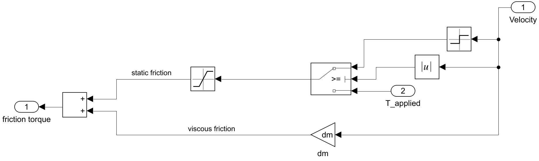
and the voltage-to-position plant is $23.94/(s^2+2.495s)$. Every controller in section 5 is designed on these two transfer functions.
2.2 Verifying the brushless motor model (application model)
The tool’s Faulhaber 3268 BX4 brushless motor was modelled as a DC-equivalent machine and checked against its datasheet before any controller was designed:
| Quantity | Datasheet | Model | Re-simulated |
|---|---|---|---|
| Stall torque | 718 mN·m | 682 mN·m | 682 mN·m (15.7 A peak) |
| No-load speed | 5500 rpm | 5268 rpm | 551 rad/s = 5262 rpm |
| Angular acceleration | 120·10³ rad/s² | 113.7·10³ rad/s² | 113.7·10³ rad/s² |
| Mechanical time constant | 4.6 ms | 4.54 ms | 4.6 ms |
2.3 Drive train with gearbox and joint
The drive-train model has four states (motor and nut angles and speeds), coupled by the gearbox stiffness (739 N·m/rad) and damping. A 1 V step gives 19.56 rad/s at the motor and 0.2415 rad/s at the nut. The gearbox mode turns out to be very stiff and overdamped, so for control the drive train behaves almost as one rigid inertia.
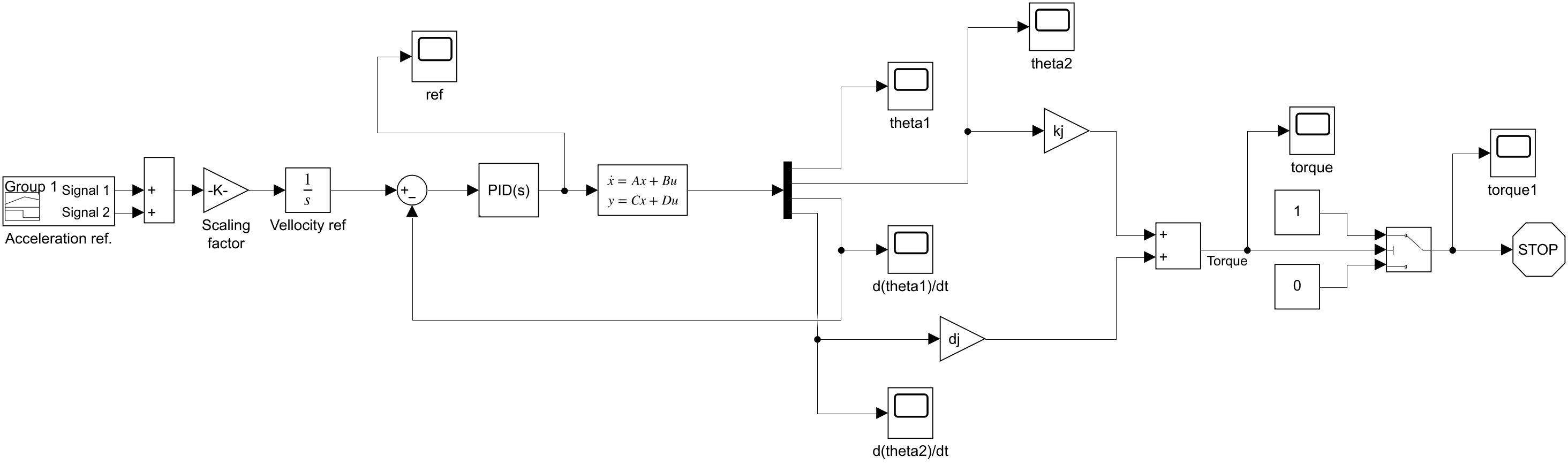
Two unit errors found by re-running the model.
statespace_screw.musesKt(gearbox stiffness, 739 N·m/rad) in the input matrix where the torque constantkt(0.0435 N·m/A) belongs, which makes the actuator gain about 17 000 times too large.- The same file uses
kj(axial bolt stiffness, 7.7·10⁷ N/m) where the rotational stiffnesskrs(3.04 N·m/rad) belongs.
Both errors appear immediately in a unit check. Lesson: check the units of every matrix entry before trusting a simulation.
3. Power stage
3.1 PWM generation on the STM32
At 40 MHz, TIM3 with ARR = 2000 produces 19.99 kHz PWM on PB4 (clockwise) and PA7 (counter-clockwise) with 2001 duty steps. That is about 11 bits, or 6 mV per step on a 12 V bridge. The motor command convention is ±2·10⁹ ↔ ±100 % duty:
/* Drive the motor in both directions: +/-2e9 <=> +/-100 % duty */
void Peripheral_PWM_ActuateMotor(int32_t con)
{
    con = con/1000000;                    /* -> +/-2000 compare counts (ARR = 2000) */
    if (con > 2000)  {con = 2000;}
    if (con < -2000) {con = -2000;}
    if (con > 0) { TIM3->CCR1 = con; TIM3->CCR2 = 0; }      /* CW  */
    if (con < 0) { TIM3->CCR1 = 0;   TIM3->CCR2 = -con; }   /* CCW */
}
PWM against the winding. The coreless motor’s electrical corner, $R/(2\pi L)=2.6$ kHz, is only 7.7 times below the PWM frequency. At stall and 50 % duty that leaves 0.71 A of current ripple, on a motor rated 0.48 A continuous.
The missing zero. The specification required “motor stationary if value is 0”. With con == 0 neither branch runs, so the previous duty stays applied. The distributed version’s failure path writes TIM3->CCR1 = 0; TIM3->CCR2 = 0; directly, next to a commented-out Peripheral_PWM_ActuateMotor(0), which is consistent with this having been discovered in testing.
3.2 Supply board (24 V → 12 V / 5 V)
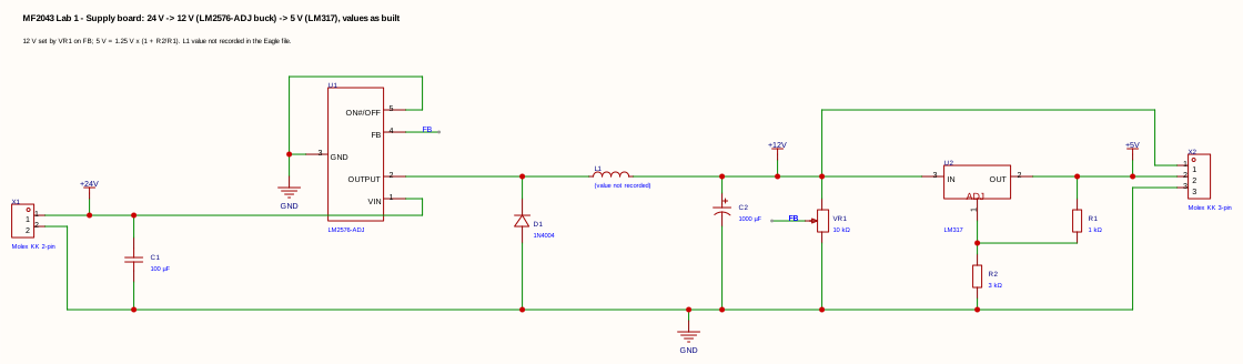
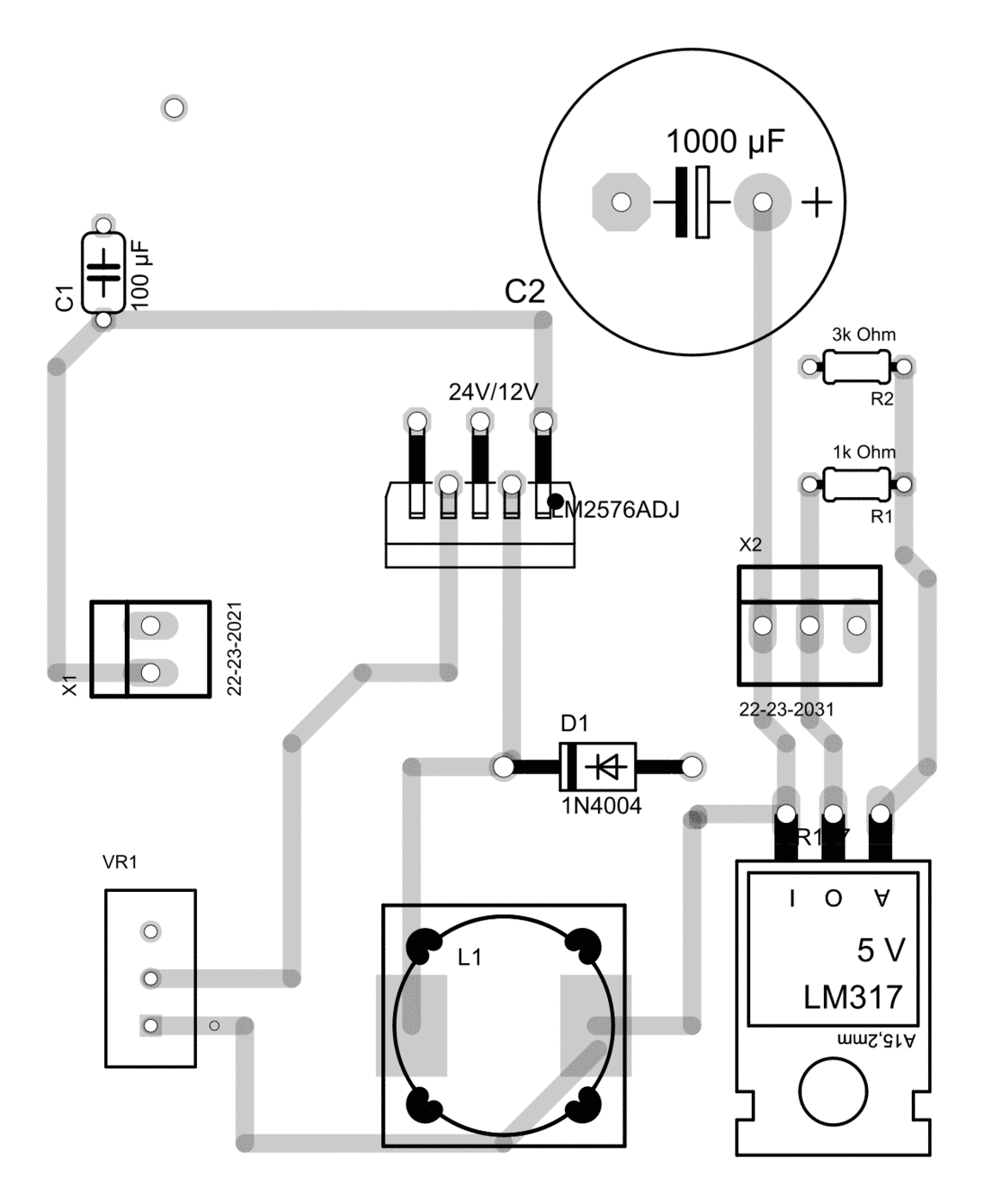
| Net | Connections |
|---|---|
| +24 V | input connector, $C_1$ (100 µF), LM2576 $V_{\text{IN}}$ |
| switch node | LM2576 output, catch diode $D_1$ (1N4004) cathode, inductor $L_1$ |
| +12 V | $L_1$, $C_2$ (1000 µF), LM317 input, trimmer $VR_1$ (10 kΩ) top, output connector |
| feedback | LM2576 FB to the $VR_1$ wiper (adjustable 12 V) |
| +5 V | LM317 output, $R_1$ (1 kΩ), output connector; ADJ node $R_1$/$R_2$ (3 kΩ) to ground: $V_{\text{out}}=1.25(1+3/1)=5.0$ V |
Review notes (as drawn).
- The catch diode is a standard-recovery 1N4004, but a 52 kHz buck regulator needs a Schottky diode (e.g. 1N5822).
- The LM317 divider draws 1.25 mA, below the regulator’s 3.5-10 mA minimum load. Datasheet designs use $R_1$ = 120-240 Ω.
- The inductor value is not recorded in the file.
3.3 H-bridge board (A4973) and solenoid driver
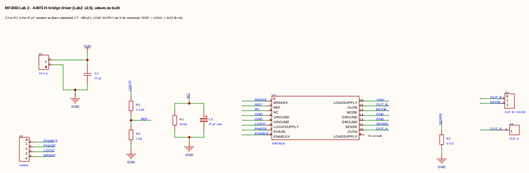
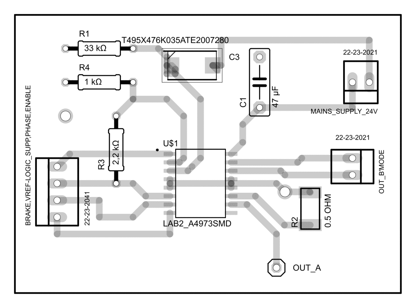
| Pin / net | Connection | Function |
|---|---|---|
| LOAD SUPPLY | +24 V, $C_1$ 47 µF | motor supply ($V_{BB}$ ≤ 50 V) |
| OUT A, OUT B | motor connectors | bridge outputs |
| SENSE | $R_2$ = 0.5 Ω to ground | current sense |
| REF | divider $R_3$ = 2.2 kΩ (from logic supply) / $R_4$ = 1 kΩ | $V_{\text{REF}}=0.3125\,V_{CC}$ |
| RC | $R_1$ = 33 kΩ ∥ $C_3$ (to ground) | fixed off-time $t_{\text{off}}=R_TC_T$ |
| BRAKE, PHASE, ENABLE | 4-pin header with logic supply | logic inputs from the MCU |
| MODE | header, beside OUT B | slow / fast decay selection |
Function and tests.
- Control pins: PHASE selects the direction, ENABLE switches the outputs, MODE selects slow or fast decay, and BRAKE shorts the motor through both low sides.
- Current limit: the internal chopper limits the current to $I_{\text{trip}}=V_{\text{REF}}/(2R_S)\approx1.03$ A with 3.3 V logic, meeting the < 1.2 A requirement.
- Bridge test: a 20 kHz PWM on PHASE drove one motor while a second motor, loaded by a power resistor, acted as a generator. The motor current was read across $R_S$ at 25 % and 75 % duty and at 1 kHz.
- Solenoid driver: a separate stage drove a 40 mH, 13 Ω solenoid with an IRFB7446 MOSFET, at 20 Hz and 20 kHz PWM, with and without a freewheel diode.
Review notes (as drawn).
- The RC pin connects to a 47 µF tantalum instead of the datasheet’s ~680 pF. That gives $t_{\text{off}}\approx1.55$ s instead of about 20 µs, so every current-limit trip would switch the bridge off for 1.5 s.
- With 5 V logic, $V_{\text{REF}}=1.56$ V exceeds the 0-1 V reference range.
- There is no ceramic decoupling at the supply pins, and the only bulk capacitor (47 µF) sits at the datasheet’s minimum recommendation (> 47 µF, close to the device).
- The datasheet’s block diagram has two LOAD SUPPLY (VBB) terminals, pins 9 and 16; as drawn only pin 16 is connected, so all bridge current enters through one pin. Connect both.
- A DAC on REF would turn the chopper into a programmable hardware current controller.
4. Sensing and the signal chain
4.1 Encoder interface and speed estimate
On Rig B, TIM1 counts the encoder’s A/B edges in hardware (×4 quadrature) into a 16-bit counter that the control loop simply reads (return TIM1->CNT;). Speed comes from the difference of two readings over the control period (the M-method):
int16_t rad = encoder - oldencoder;          /* signed 16-bit difference: wrap-safe */
vel_cal = -rad*60/dt*1000/2048;              /* rpm, 2048 counts/rev assumed        */
At 2000 rpm and 50 ms about 3413 counts pass, and one count is worth 0.59 rpm. At a 1 kHz loop rate one count would be 29.3 rpm, too coarse for a speed loop. The 2048 counts/rev constant is not documented anywhere; a wrong value would be a silent gain error on speed. Rig A used plsPerRev = 3600 at 2 ms, which gives 0.87 rad/s per count.
Simulated improvement. A Kalman filter that fuses the counts with the motor current and model removes the quantization without filter lag, and it estimates the load torque. Here it is compared with the alternatives on the Rig B motor model:
4.2 Anti-alias filters and sampling
A separate board set built filters for a microcontroller ADC designed for $f_s=8$ kHz. Test signals at $f_c/3$, $f_c$ and $3f_c$ were sampled on an mbed LPC11U24 and streamed to MATLAB, and digital 200 Hz low-pass and 600 Hz high-pass filters were implemented.
| Filter | Values | Cut-off | Note (as drawn) |
|---|---|---|---|
| Passive RC | 0-10 kΩ trimmer, 100 µF | ≥ 0.16 Hz | far too low; $f_c\approx0.3f_s=2.4$ kHz needs about 6.8 nF with 10 kΩ |
| Active low-pass (OP462) | inverting, 10 kΩ in, 100 kΩ ∥ 10 nF | 159 Hz, gain −10 | inverts and amplifies a 0-3.3 V signal; the op-amp’s hidden V+ pin shares the input net and V− is unconnected |
| Passive band-pass | 100 nF, 200 Ω, 400 Ω, 47 nF | corners 8.0 / 8.5 kHz | loaded stages: peak −7.6 dB at 8.2 kHz, −3 dB band 2.9-23 kHz |
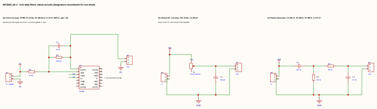
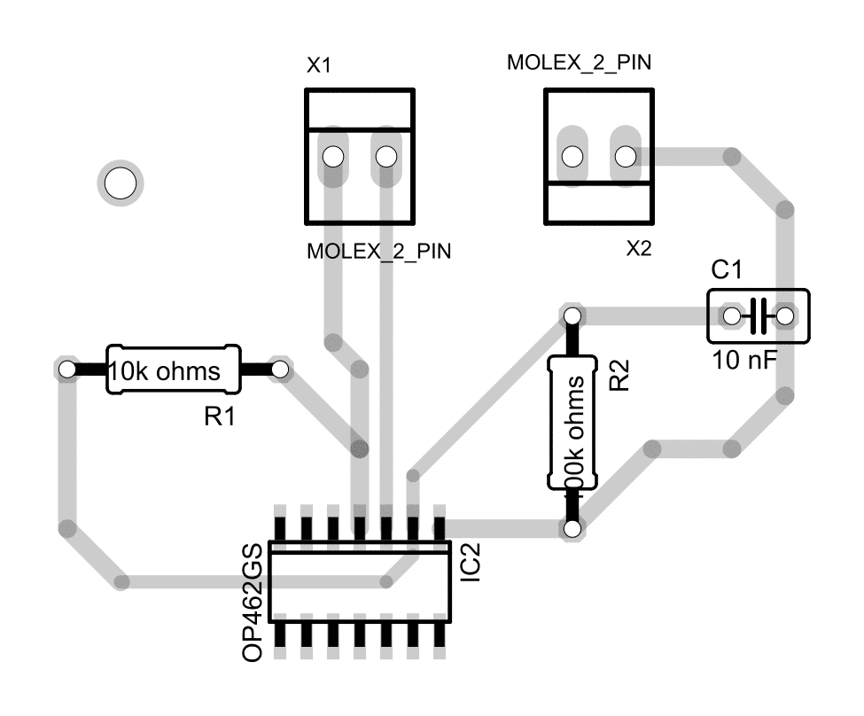
Three sampling frequencies. The filter specification uses 8 kHz, the sampling program 20 kHz (one byte per sample at 921 600 baud) and the MATLAB plotter 80 kHz. Used together unchanged, every plotted frequency reads four times too high. Lesson: define $f_s$ once and store it with the data.
4.3 Current sensor board
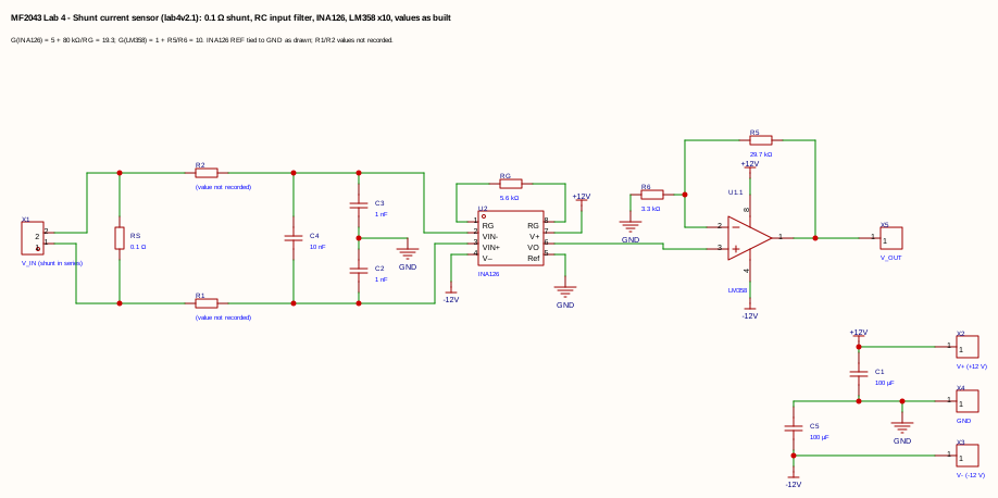
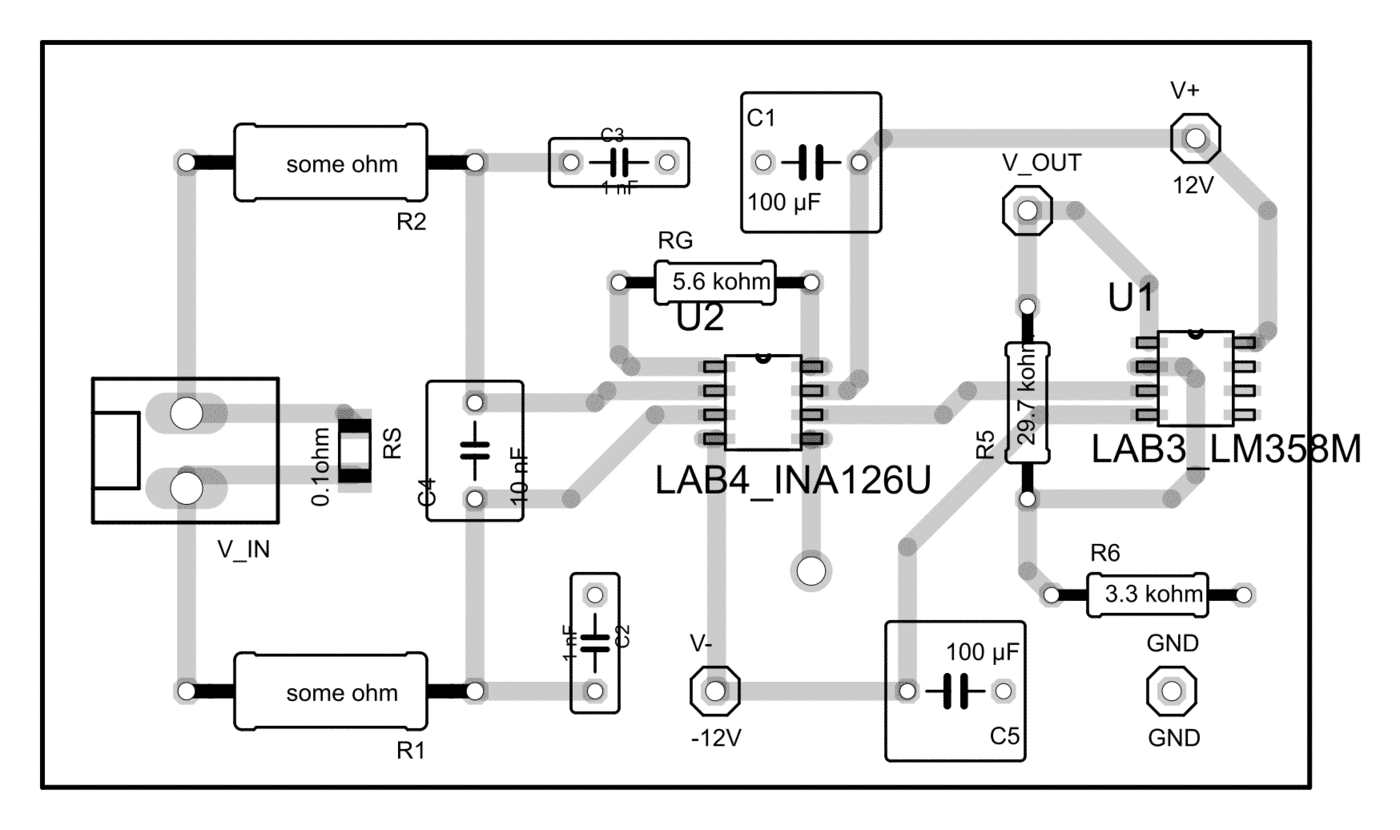
Signal chain.
- A 0.1 Ω shunt in series with the motor.
- An RC input filter: series resistors, 1 nF common-mode and 10 nF differential capacitors.
- An INA126 instrumentation amplifier with $G=5+80\ \text{k}\Omega/5.6\ \text{k}\Omega=19.3$ (roughly 45 kHz bandwidth at this gain).
- An LM358 stage with gain ×10.
Tests. The sensor was calibrated against known currents, its output was recorded with the motor on DC and on PWM, and the signal-to-noise ratio was measured before and after low-pass filtering.
Review notes (as drawn).
- At 19.3 V/A the output saturates near ±0.55 A, and a 0-3.3 V ADC sees only 0-0.17 A.
- The REF pin is grounded, so negative currents are lost.
- Designing backwards from the ADC gives about 1.1 V/A around a buffered, ratiometric 1.65 V.
- In-line placement exposes the amplifier to the full PWM common-mode swing. Low-side placement or a PWM-rejecting current-sense amplifier avoids that.
PWM ripple and the sampling instant. Whichever sensor is used, the current must be sampled synchronously with the PWM, at the point where the ripple crosses its average:
5. Control design and results on hardware (Rig A)
5.1 Speed control
Design. The PI was designed by pole placement for no overshoot ($\zeta=0.946$) and 0.2 s settling ($\omega_0=24.3$ rad/s), giving $K_p=1.82$ and $K_i=24.7$. It was implemented as a two-degree-of-freedom controller with the reference entering only through the integrator, so a step does not kick the proportional term. Discretized with Tustin at $T_s=2$ ms:
\[u(z)=\frac{0.02467z+0.02467}{z-1}\,r(z)-\frac{1.842z-1.793}{z-1}\,y(z).\]Measured.
- A 50 rad/s step settled without overshoot, within the 1 rad/s error requirement.
- A reference of $50\sin(2\pi\cdot0.2t)$ was tracked.
- Stopping the motor by hand under the sine drove the voltage to the ±24 V rails, alternating at the reference frequency.
5.2 Position control
Design. A polynomial (RST) controller placed the dominant poles at 12 rad/s ($\zeta=1$) and the observer poles at 30 rad/s ($\zeta=0.8$):
\[\frac{S(s)}{R(s)}=\frac{29020s^2+409100s+1859000}{s^2+69.5s},\qquad \frac{T(s)}{R(s)}=\frac{2066s^2+99170s+1859000}{s^2+69.5s}.\]Measured.
| Design | $T_s$ | Overshoot | Rise time | Remark |
|---|---|---|---|---|
| Continuous design, Tustin emulation | 2 ms | 1.7 % | 0.54 s | back-calculation anti-windup, $K_{\text{aw}}=1/T_s=500$ |
| Direct discrete design (ZOH plant) | 50 ms | ≈ 0 % | 0.47 s | same poles mapped by $z=e^{sT_s}$ |
| Continuous design, Tustin emulation | 50 ms | – | – | fails: the fastest frequency (36 rad/s) needs 6-17 ms |
5.3 Servo control
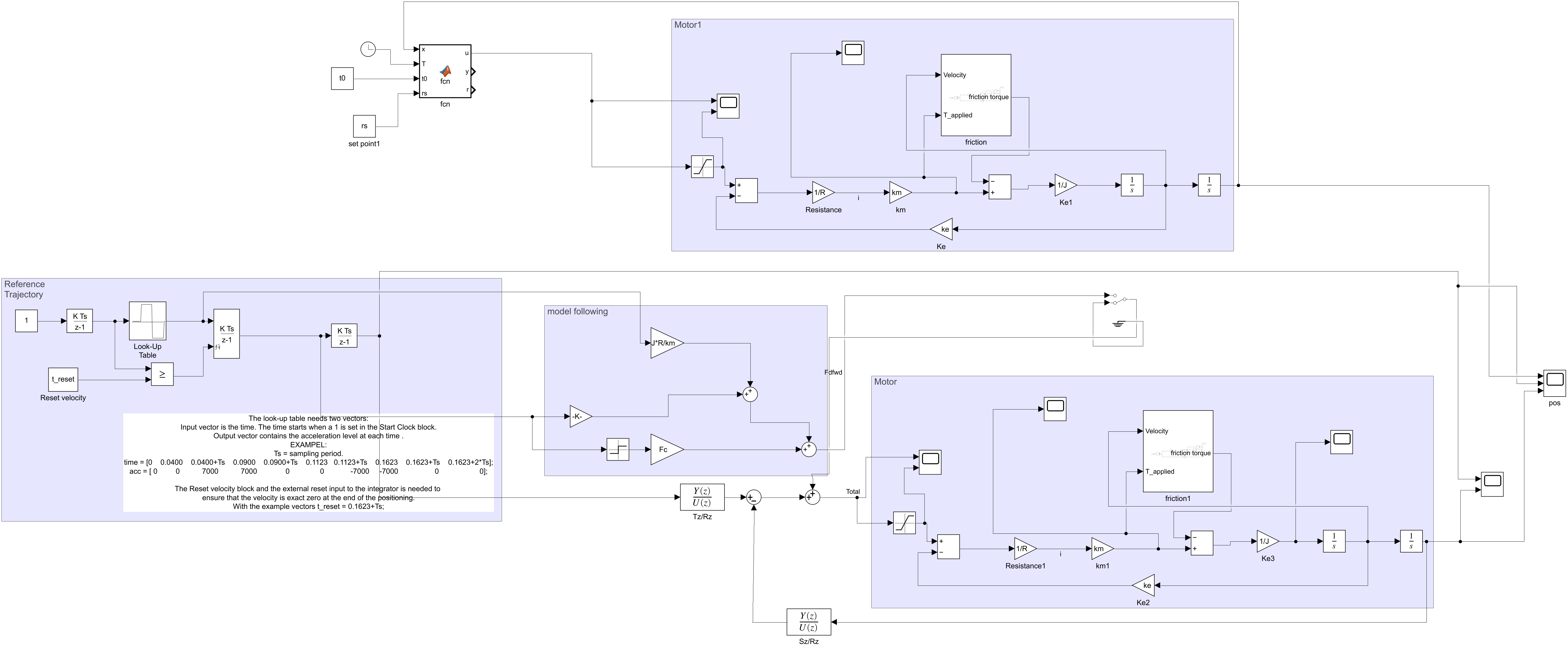
A trapezoidal trajectory planner (500 rad/s², 210 rad/s, chosen from the identified model so that the voltage never saturates) and a model-following feedforward made 10 rad and 100 rad moves with about 0.5 s rise time. The real motor tracked as well as the simulation.
5.4 Sampling, delay and saturation (re-simulated)
5.5 Robustness
The sensitivity $S$ and complementary sensitivity $T$ were compared for different observer polynomials. The same method was applied to a velocity controller for a valve-controlled hydraulic cylinder, tested against an external force, a change of load mass and sensor noise.
6. Embedded implementation (Rig B)
6.1 Firmware architecture
The firmware has four modules with fixed header files (core, peripherals, controller, application), written as if by four teams in parallel. The same PI law was run in three execution models:
- Super-loop. The loop polls
HAL_GetTick()and runs the controller whenmillisec % PERIOD_CTRL == 0; the reference toggles between ±2000 rpm every 4 s. The PI is an incremental Tustin form that receives the elapsed time, so it works at both 10 and 50 ms. - RTOS. Keil RTX (CMSIS-RTOS v1) virtual timers (50 ms and 4 s) signal a control thread and a reference thread. The HAL’s SysTick, SVC and PendSV handlers had to be removed to avoid clashing with the kernel’s.
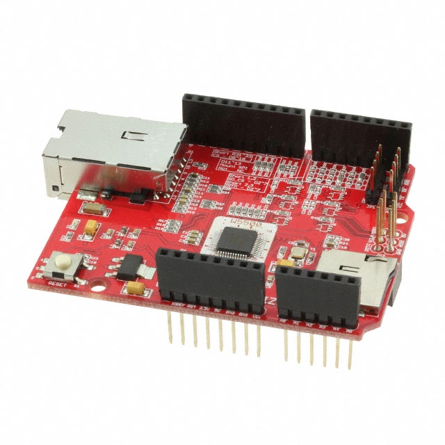
- Distributed over TCP. A client board samples the encoder and drives the motor; a server board computes the PI. Each period the client sends the speed (4 bytes,
SF_TCP_NODELAY), waits in a blockingrecv()and actuates; on failure it zeroes the PWM.
6.2 Re-executing the firmware
controller.c and peripherals.c were replayed in Python with exact C integer semantics (32-bit wrap, truncating division, the original signed/unsigned conversions) against a model of the motor. The replay assumes a 12 V supply, sign-magnitude drive, 2048 counts/rev and rotor inertia only.
Two overflow mechanisms.
- RTOS version.
ki*Iexceeds 32 bits before the clamp, and the back-calculation term(u - v)*kantis $9\cdot10^5$ times stronger than a deadbeat correction, so it overflows too. - Final version. The clamp at $\pm2\cdot10^9$ comes after the addition, leaving only $1.47\cdot10^8$ of headroom. With the rotor held at 50 ms one increment is $1.56\cdot10^8$: the sum wraps and the clamp turns it into full reverse duty. At 10 ms the increment fits.
6.3 Code review findings
| Finding | Effect | Fix |
|---|---|---|
int16_t difference of encoder readings |
handles 16-bit counter wrap correctly | keep |
-rad*60/dt*1000/2048 divides before scaling |
truncation at 50 ms | multiply first: -rad*60000/(dt*2048) |
| early draft divides by 60 instead of multiplying | speed reads 0 below 3600 rpm | unit test of the conversion |
ActuateMotor(0) leaves the previous duty |
motor not stopped by a zero command | add the else branch |
kp*t mixes int16_t and uint32_t |
computed unsigned; correct only by two’s-complement accident | explicit casts or float |
RTOS PI: ki*I and (u-v)*kant exceed 32 bits |
sign flip when the rotor is held (undefined behaviour) | int64_t/float, correct back-calculation scaling |
| final PI: clamp after the addition | full reverse duty with the rotor held at 50 ms | add in 64 bit, then clamp |
comment “every 10 ms” with PERIOD_CTRL 50 |
documentation drift | measure the period with a GPIO |
| server resets the controller from another thread | race on the integrator | reset request flag, one owner |
client recv() without timeout |
a network stall freezes the control thread | socket timeout, stale-data rule |
6.4 From control equation to torque
At the steady state of a +2000 rpm reference:
- Sensor. Every 50 ms the thread reads
TIM1->CNT; about 3413 counts have passed. - Estimate.
velocity≈ 2000 rpm. - Control. The PI holds
pidout≈ 4.1·10⁸ (20.6 % of 2·10⁹). - PWM.
TIM3->CCR1 = 412, so PB4 is high for 10.3 µs of every 50 µs. - Bridge. The shield applies 12 V for 20.6 % of each period, 2.47 V on average.
- Winding. (2.47 − 2.38 V back-EMF) / 3.42 Ω ≈ 25 mA, the no-load current, with about 0.5 A of PWM ripple.
- Torque. $k_ti$ ≈ 0.29 mN·m balances friction, and the speed holds.
7. Application study: a bolt-tightening drive (simulation)
The loop was then scaled to an application: the drive of an Atlas Copco Tensor ETV STB62-50-B10 nutrunner, with a Faulhaber BX4 brushless motor, a 9 × 9 planetary gearbox and an M8 bolted joint. The target is 25 N·m, finishing at 3 rad/s at the nut.
Gear ratio. The requirement is a constant-power curve at the motor (about 83 W), close to the motor’s 99 W peak at 24 V.
- With $n=81$ the clamp point (0.34 N·m, 243 rad/s) needs 22 V and 7.9 A, but the free speed is only about 59 rpm against the product’s 375 r/min.
- Reaching 375 r/min needs $n\le18.3$, and then the clamp needs 1.52 N·m, twice the stall torque.
The specified motor cannot meet both requirements.
Joint model. Without friction the model predicts 2.82 GPa bolt stress, far above the 640 MPa yield. With thread and under-head friction ($\mu=0.2$), 25 N·m gives 11.7 kN of preload and 321 MPa, reached about 44° after snug.
Stopping at the target. If the drive keeps commanding the clamp torque and lets the joint stop the rotor, the rotor’s 0.18 J of kinetic energy winds the joint a further 0.11 rad: 3.5 N·m (14 %) overshoot. Cutting the current exactly at the target gives about 0.2 N·m, but then every millisecond of torque-measurement delay adds 0.1 N·m. Slowing to 0.5 rad/s before the target brings the torque-limited overshoot down to 0.6 N·m, which is why production tools tighten in two steps.
Energy. After the unit errors of section 2.3 are fixed, the clamp phase alone needs about 20 J: 7.7 J of copper loss, 10.7 J of mechanical work and about 1 J of no-load losses. The original model gave 140 J per tightening and about 2000 bolts per 2.6 Ah charge.
8. Brushless drive shields for the BX4 (design)
The application study showed what a real tool drive needs: a three-phase bridge for the BX4, about 8 A at the clamp point, current measurement and a speed estimate that works at low speed. Both rigs in this project drive brushed motors through H-bridges, so the next hardware step is a pair of Nucleo-L476RG shields for the BX4. Both are built around the same power stage:
- a TI DRV8323S gate driver (6-60 V, SPI-configured, three integrated current-sense amplifiers);
- six Infineon BSC028N06NS 60 V MOSFETs (2.8 mΩ);
- a 24 V input with an SMBJ33A TVS, bulk capacitors and decoupling on each bridge leg.
They differ in how the motor is commutated and in what is measured. That makes them the hardware versions of the velocity loop and the torque loop in the theory post (Parts E, G and I).
| Velocity shield | Torque shield | |
|---|---|---|
| DRV8323S mode (set over SPI) | 1×PWM: INHA = PWM, INLA/INHB/INLB = Hall A/B/C, INHC = DIR, INLC = nBRAKE | 3×PWM: INHx = TIM1 CH1-3, INLx = common enable |
| Commutation | six-step, inside the driver, from the Hall states | sinusoidal, in firmware (FOC), from the encoder angle |
| Current sensing | one 5 mΩ DC-link shunt → CSA A | three 5 mΩ low-side phase shunts → CSA A/B/C |
| Position sensing | Hall A/B/C (4.7 kΩ pull-up, 1 kΩ/1 nF filter) → TIM3/TIM2 input capture | incremental encoder A/B/I (4.7 kΩ pull-up, 330 Ω/100 pF filter) → TIM3 encoder mode; Halls for start-up alignment |
| Firmware loop | speed PI with anti-windup, duty clamp and current limit | Clarke → Park → PI on $i_d$, $i_q$ → inverse Park → SVPWM, once per PWM period |
| PCB status | draft: a few connections still unrouted | routed |
8.1 Velocity shield: six-step with Hall commutation
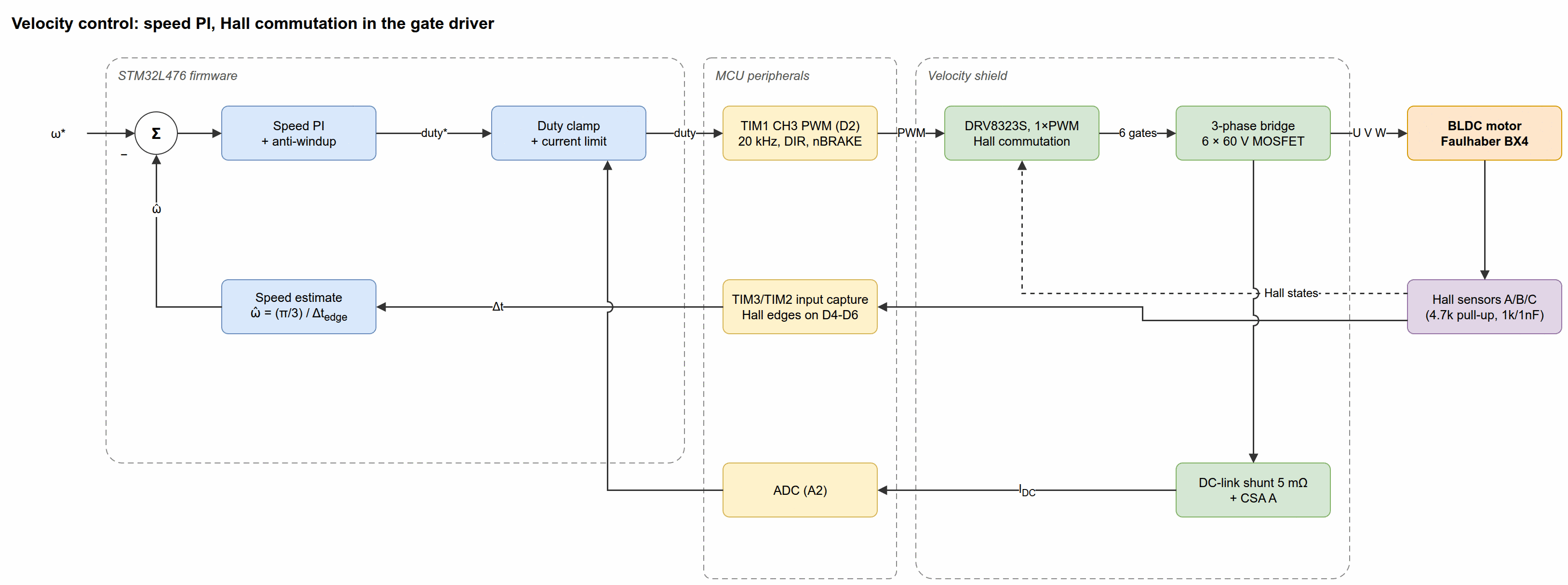
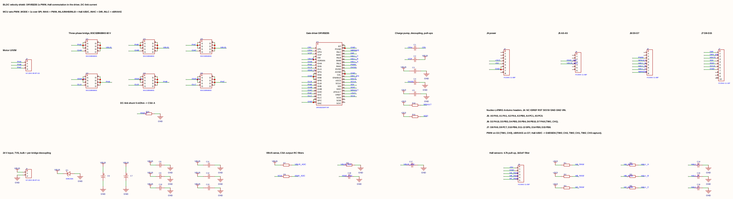
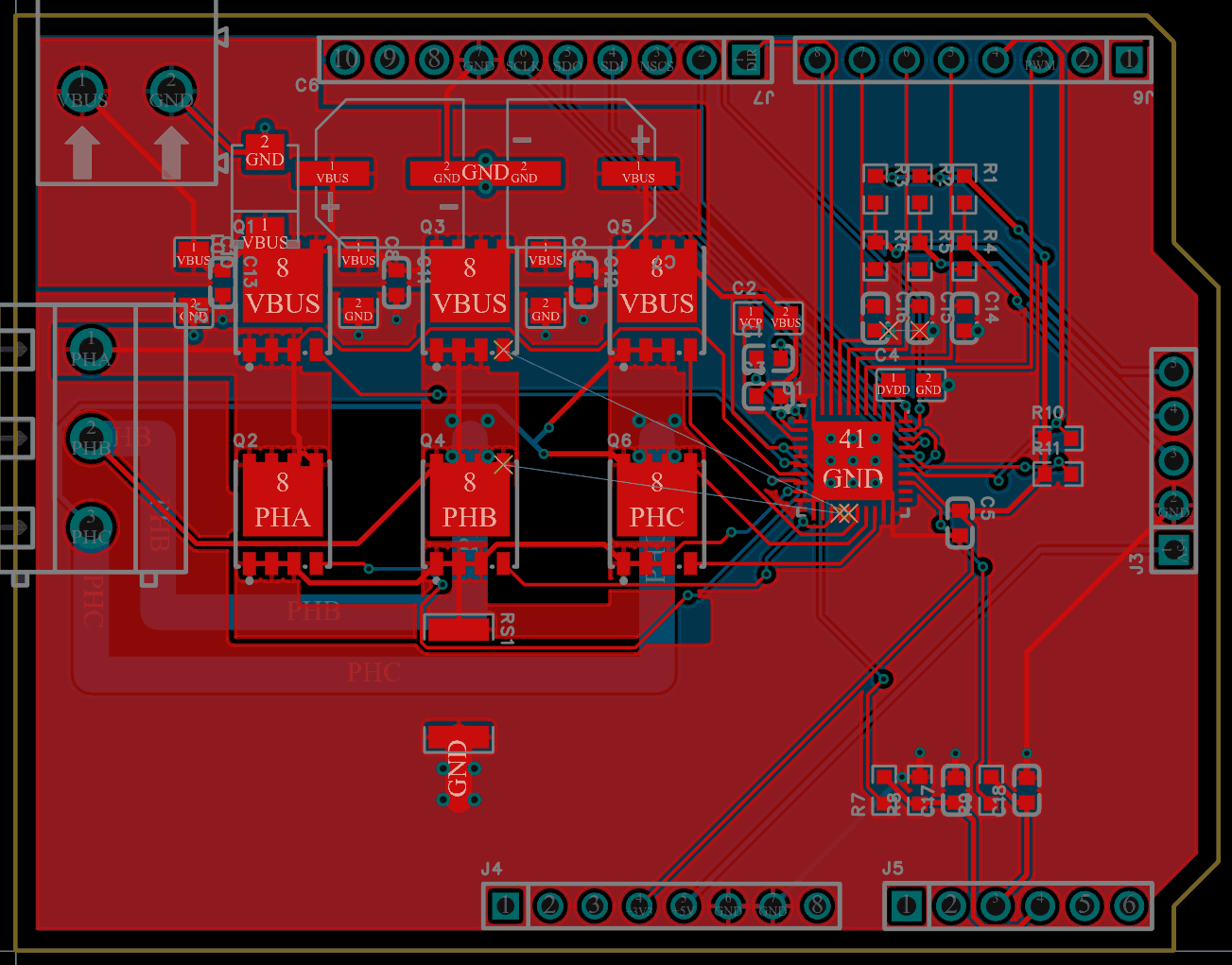
Design notes.
- Speed from Hall edges. The speed comes from timing the Hall edges (the T-method of Part E.5): $\hat\omega_e=(\pi/3)/\Delta t_{\text{edge}}$. With two pole pairs that is 12 edges per mechanical revolution. At the clamp speed (243 rad/s) an edge arrives every 2.15 ms, so a 1 MHz capture clock resolves 0.05 %. The estimate is fresh only once per edge, about 465 times a second at clamp speed and much less near standstill, where a timeout must declare zero speed. A 1 kHz speed loop therefore sees a sampling rate that changes with speed.
- DC-link current. The DC-link shunt carries the conducting phase current only during the PWM on-time. The current-limit sample belongs in the middle of the on-time, triggered by the PWM timer.
8.2 Torque shield: FOC with three-shunt sensing
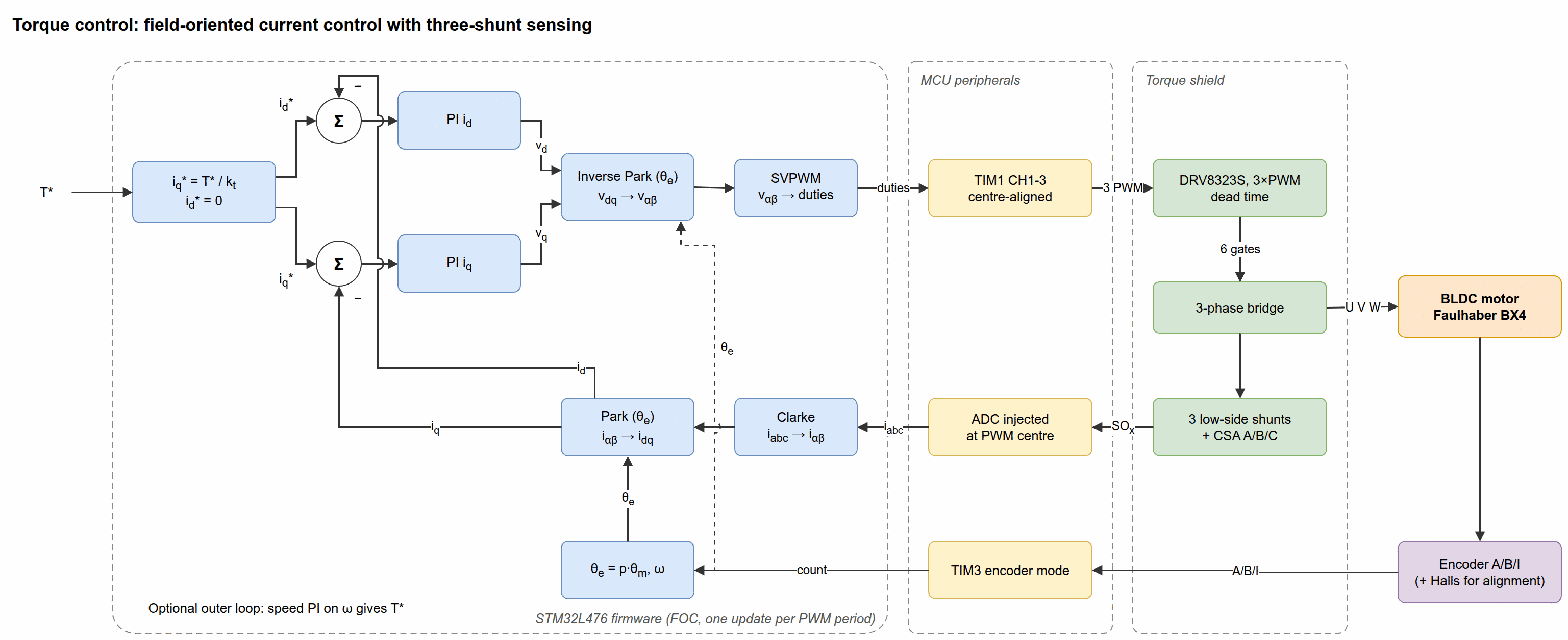
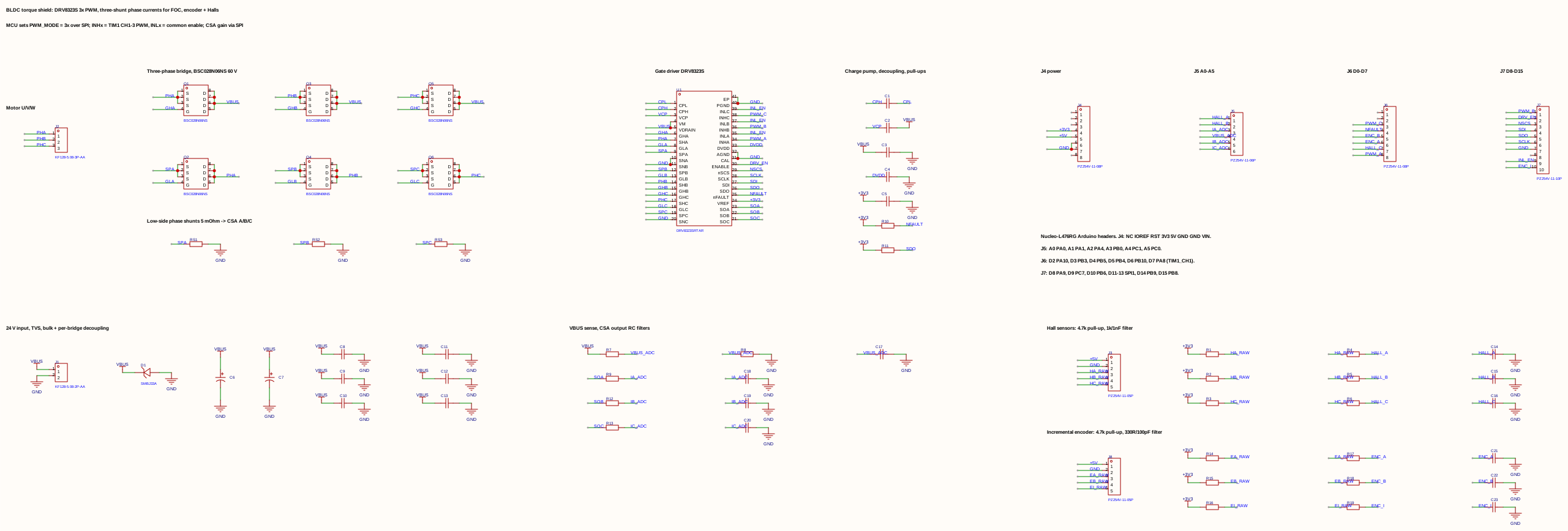
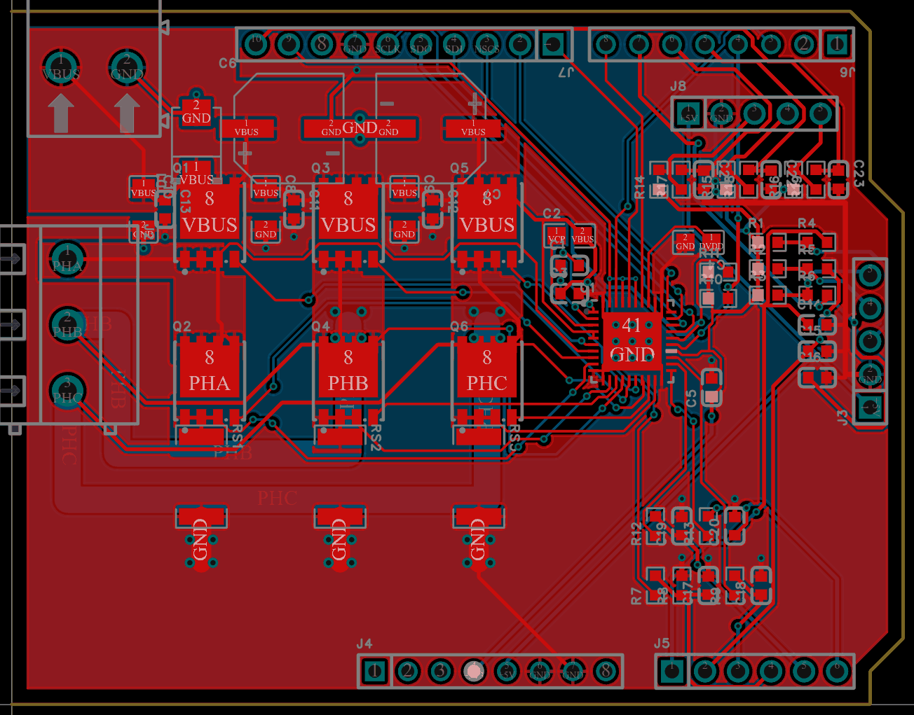
Design notes.
- Current range. The DRV8323S amplifiers are bidirectional around $V_{\text{REF}}/2$, with gains of 5, 10, 20 or 40 V/V. With 5 mΩ and a gain of 20, a 3.3 V ADC covers ±16.5 A at 8 mA per LSB. That is two times headroom over the 7.9 A clamp current, and the design follows the “backwards from the ADC” rule (Part E.4) that the old lab sensor missed.
- When to sample. Low-side shunts see a phase current only while that leg’s low-side MOSFET conducts. With centre-aligned PWM all three low sides conduct in the zero vector at the centre of the period, which is why the ADC is injected there (Part F.1).
- Losses. At 7.9 A each shunt dissipates 0.31 W and each conducting MOSFET about 0.17 W.
- Input filters. The Hall filter (1 kΩ, 1 nF, $\tau$ = 1 µs) and the encoder filter (330 Ω, 100 pF, $\tau$ = 33 ns) reject nanosecond spikes while passing edge rates of hundreds of kHz and several MHz respectively.
8.3 Open points before ordering
- Unannotated values. The values of the CSA output filters, the bus-voltage divider and the charge-pump and decoupling capacitors are not shown on the schematics yet. Their cut-off and attenuation must be checked against the 20 kHz PWM and the ADC sampling time (Part F.3).
- Regenerative braking. Stopping the BX4 from no-load speed on a 24 V bench supply with 470 µF of bus capacitance would push the bus to about 70 V (Part J.4 of the post), above the 60 V MOSFETs and the DRV8323S supply range. The TVS is meant for short transients, not for absorbing braking energy, so braking needs a current limit on regeneration or a brake chopper.
- Battery voltage. The SMBJ33A’s 33 V stand-off suits a 24 V supply but is marginal for a fully charged battery pack above 33 V.
- SPI clock and the LED. SPI1 uses D11-D13; D13 (PA5) also drives LED LD2, which will flicker with the SPI clock. That is harmless.
- Velocity shield routing. Its PCB still needs the remaining connections routed and a design-rule check.
8.4 Reference Simulink models of both drives
Before any firmware for the shields, both drive types were simulated in Simulink with the BX4 constants of the application study, the 20 kHz control period of the STM32 firmware and the same speed loop, so they can be compared like for like. The model files are not published here; only the structure and the results are.
| Quantity | Value | Source |
|---|---|---|
| Supply, current limit | 24 V, 7.9 A | clamp point of section 7 |
| Pole pairs, inertia | 2, 6·10⁻⁶ kg·m² | project data, $b=0$ |
| Terminal resistance, inductance | 1.45 Ω, 110 µH | project data |
| Torque constant | 43.5 mN·m/A | project data |
| PMSM equivalent | $R_s=R_{ll}/2$, $L_d=L_q=L_{ll}/2$, $\lambda=k_t/(1.5p)$ | so that $T_e=1.5p\lambda i_q=k_ti_q$ |
| Control period | 50 µs (20 kHz), one sample of computation delay | firmware of section 8 |
| Current loop | PI by pole-zero cancellation, 1 kHz | $k_p=\omega_cL$, $k_i=\omega_cR$ |
| Speed loop | PI, 60 Hz, output limited to 7.9 A with clamping anti-windup | $k_p=J\omega_c/k_t$, $k_i=k_p\omega_c/5$ |
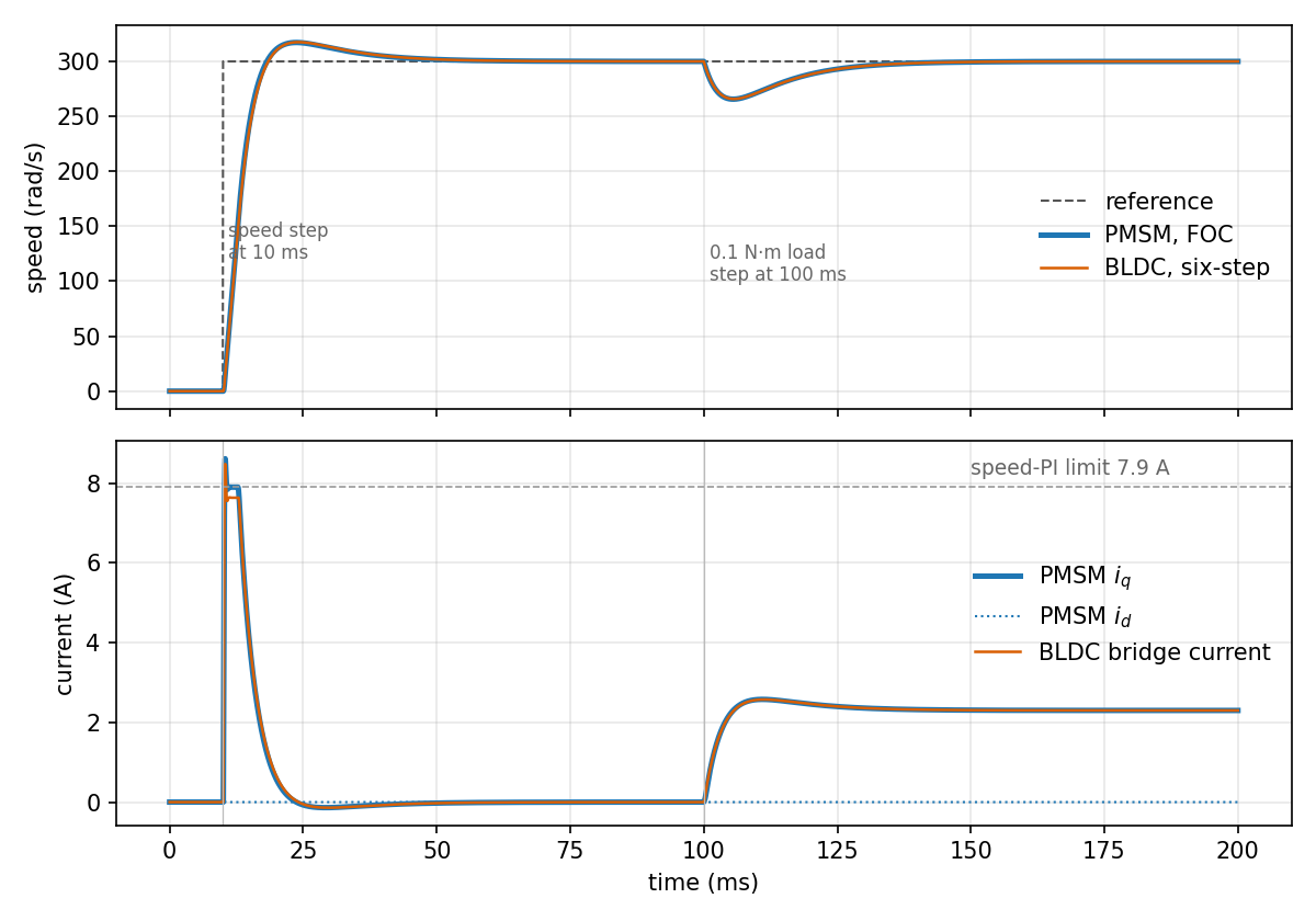
PMSM with field-oriented control (simulated structure). The speed PI sets $i_q^$ ($i_d^=0$). Two current PIs work in the rotating frame with the cross-coupling and back-EMF feed-forward terms $-\omega_eL_qi_q$ and $\omega_e(L_di_d+\lambda)$. The voltage vector is scaled back onto the circle $V_{dc}/\sqrt3$ (the linear SVPWM limit), delayed one sample and rotated back to the stator frame. The plant is the dq model; $i_a$ and $i_b$ are rebuilt from it and pass through Clarke and Park again, as a three-shunt measurement would.
BLDC with six-step commutation (simulated structure). The speed PI sets the bridge current reference and a current PI sets the signed duty. The rotor angle is converted to degrees and shifted, wrapped with a mod block and compared with 180° to give the three Hall bits (edges at 30° + k·60°). A Combinatorial Logic block holds the six-step truth table (Hall code in, six gate signals AH, AL, BH, BL, CH, CL out). In parallel, three lookup tables give the trapezoidal back-EMF shapes $f_a,f_b,f_c$ of the three phases, and the gate signals select the conducting pair: $s=\tfrac12\sum_x(H_x-L_x)f_x$. The plant is the lumped model of the two conducting phases: $L_{ll}\,di/dt=v-R_{ll}i-k_es\omega$ and $T_e=k_ts\,i$. In the flat part of the trapezoid $s=1$; the ramps of the shapes appear only around the commutation instants.
Simulated response. A 300 rad/s step at 10 ms and a 0.1 N·m load step at 100 ms (the plots end at 200 ms):
| PMSM, FOC | BLDC, six-step | |
|---|---|---|
| 90 % rise time | 6.0 ms | 6.2 ms |
| Overshoot | 5.7 % | 5.8 % |
| Settling to 2 % | 27.9 ms | 28.6 ms |
| Speed dip at the load step | 34 rad/s | 34 rad/s |
| Recovery to 2 % | 26.5 ms | 26.6 ms |
| Peak current | 8.6 A ($i_q$) | 8.5 A |
| Steady-state current at 0.1 N·m | 2.30 A, $i_d\approx0$ | 2.30 A |
What these models do not contain. Both use an average-value inverter, so there is no PWM ripple, dead time, MOSFET drop or bus-voltage sag, and no sensor noise or quantisation. The rotor angle and speed are the plant states, not the Hall-edge T-method estimate of section 8.1. Friction is $b=0$, as in the project data. The PMSM flux linkage is derived from the torque constant by assuming a sinusoidal machine, which the BX4 only approximates. The BLDC model lumps the two conducting phases and ignores the freewheeling phase, so torque ripple at commutation is understated. None of this has been checked against the shields, which are not built.
9. Results and lessons
| Area | Result |
|---|---|
| Identification | DC-motor parameters from steps and sines; Coulomb friction needed for low-voltage accuracy |
| Speed control | no overshoot, ≤ 1 rad/s error on hardware; saturation observed at ±24 V |
| Position control | 1.7 % overshoot, 0.54 s rise at 2 ms; direct discrete design at 50 ms: ≈ 0 %, 0.47 s |
| Embedded speed control | ±2000 rpm tracked at 10 and 50 ms periods in super-loop, RTOS and distributed versions |
| Electronics | supply, H-bridge, filters and current sensor built; review found off-time, range, supply-pin and decoupling issues |
| BLDC shields | velocity (six-step, Hall) and torque (FOC, three shunts) shields designed around the DRV8323S; torque PCB routed |
| Re-execution | 2 unit errors in the model, 3 overflow/actuation bugs in the firmware, 1 infeasible requirement |
Lessons.
- Design the sensor backwards from the ADC, and the sampling instant from the PWM.
- Choose the sampling period from delay, not from habit. A direct discrete design survives periods that break an emulated one.
- Every loop saturates. Anti-windup and arithmetic headroom must be tested with a stalled rotor, not only with a step.
- Units are the cheapest test. Every serious error found here was a unit or range mismatch between two pieces written separately.
- Re-execute old work. Re-running models and firmware against each other found more than re-reading them did.
10. Next steps
- Finish the BLDC shields. Annotate the remaining values, route the velocity shield, run design-rule checks, then order and bring up the velocity shield first (simpler firmware, Hall commutation in the driver).
- Firmware for the shields:
- a speed PI on Hall-edge timing for the velocity shield;
- FOC with PWM-centred ADC sampling for the torque shield;
- the Kalman speed estimator of section 4.1 on the encoder.
- Fix the Rig B firmware: add in 64 bit before clamping, add the zero-duty branch, correct the back-calculation scaling, and test the stalled rotor on hardware.
- Port to Zephyr on the same Nucleo board.
Provenance table
Status codes: B built and tested · M measured on hardware · Mo modelled/simulated · D datasheet · R re-derived for this page · A assumed · U unknown (not in any surviving file).
| Element | Value | Source | Status |
|---|---|---|---|
| Rig A | |||
| Controller board | TI LAUNCHXL-F28379D (dual C28x, 200 MHz), Simulink external mode | workshop files | B |
| Motor (as used in the models) | $R$ = 112 Ω, $L$ = 11.4 mH, $k_m$ = $k_e$ = 0.0697 | initPar.m |
D (datasheet missing) |
| Identified mechanics | $J$ = 2.6·10⁻⁵ kg·m², $d_m$ = 2.15·10⁻⁵ N·m·s/rad, $F_c$ = 1.35·10⁻³ N·m | workshop report | M |
| Encoder, supply | plsPerRev = 3600; ±24 V |
initPar.m |
D |
| Sampling | 2 ms (speed, position), 50 ms (direct design) | report, initPar.m |
B |
| Rig B | |||
| MCU board | Nucleo-L476RG (Cortex-M4F), 40 MHz | CubeMX .ioc |
B |
| Motor | Assun AM-CL1643MB-1210 coreless DC, 12 V, 3.42 Ω, 0.21 mH, 11.4 mN·m/A, 3.11 g·cm², $\tau_m$ = 8.2 ms | datasheet | D |
| Driver shield | dual half-bridge; part number, supply voltage | – | U |
| PWM | TIM3 CH1 (PB4) / CH2 (PA7), ARR 2000 → 19.99 kHz | .ioc, peripherals.c |
B |
| Encoder | TIM1 encoder mode on PA8/PA9, 16-bit; 2048 counts/rev used in code | controller.c |
B / A |
| Control | PI, 10 or 50 ms period, ±2000 rpm square wave every 4 s | application.c |
B |
| Networking | WIZnet W5500 on SPI3, TCP client/server | sources | B |
| Bridge supply for replays | 12 V | – | A |
| Custom boards | |||
| Supply | 24 V → 12 V (LM2576-ADJ, 52 kHz) → 5 V (LM317) | lab1_test2.sch |
B |
| H-bridge | Allegro A4973, $R_S$ = 0.5 Ω, $I_{\text{trip}}$ ≈ 1.03 A at 3.3 V logic | Lab2_v2.5.sch |
B (as drawn) |
| Filters | passive RC, active OP462, passive band-pass; mbed LPC11U24 sampling | lab3_*.sch, course code |
B (as drawn) |
| Current sensor | 0.1 Ω shunt, INA126 (G = 19.3), LM358 (×10), ±12 V | lab4v2.1.sch |
B (as drawn) |
| Current-sensor input resistors | “some ohm” in the schematic | – | U |
| BLDC shields | |||
| Gate driver, bridge | TI DRV8323S; 6 × Infineon BSC028N06NS (60 V, 2.8 mΩ); SMBJ33A TVS | shield schematics | designed |
| Current sensing | velocity: one 5 mΩ DC-link shunt; torque: three 5 mΩ low-side shunts; CSA gain | shield schematics | designed / A (gain 20) |
| Filter, divider and capacitor values | not annotated on the schematics | – | U |
| Application model | |||
| Tool | Atlas Copco Tensor ETV STB62-50-B10: 15-50 N·m, 375 r/min, 30 V Li-ion 2.6 Ah | product sheet | D |
| Motor | Faulhaber 3268 G 024 BX4: $R$ = 1.45 Ω, $L$ = 110 µH, $k_t$ = 43.5 mN·m/A, $J$ = 60 g·cm², 2 pole pairs | datasheet | D |
| Drive train | ratio 81 (9 × 9); stiffness 739 N·m/rad, damping 1.5 N·m·s/rad; $J_i$ = 6.20·10⁻⁶, $J_o$ = 5.63·10⁻⁶ kg·m² | report, inertia.m |
Mo |
| Joint | M8 × 1.25, class 8.8; 3.04 N·m/rad without friction, 32.6 N·m/rad with friction | report / this page | Mo / R |
| Gear efficiency | 0.9 | – | A |
| Real tool gear ratio and efficiency | – | – | U |
Credits and sources
The work was done during my master’s at KTH:
- Rig A: workshops in MF2007 Dynamics and Motion Control, with Huanyu Chen and Jiahao Wang; course responsible Lei Feng.
- Rig B: the group project in MF2103 Embedded Systems for Mechatronics, under Jad El-khoury and Martin Törngren.
- Boards: individual labs in MF2043 Mechatronic Electronics; the sampling code and plotter were provided by the course.
- Application model: the MF2030 Mechatronics group project “An Electric Nut-Runner for Tightening of Bolted Joints”, with Gowtham Raj Rangaraju and Pak Chuen Hau.
Datasheets: Assun AM-CL1643MB-1210; Faulhaber 3268 G 024 BX4; Allegro A4973; TI LM2576, LM317, INA126; STMicroelectronics RM0351, UM1724; Atlas Copco Tensor STB product sheets.
Images: Nucleo-L476RG and W5500 shield from the Zephyr Project documentation (Apache-2.0); C2000 LaunchPad set-up by Brihaspati (CC BY-SA 4.0) via Wikimedia Commons. Diagrams and plots are my own; simulations and code replays were re-run in Python for this page.