Motors in the Loop: Actuators, Sensors, Models, Controllers and Sensor Fusion
These are my course notes on one question: how a motor becomes a controlled actuator. They draw on four KTH courses: MF2030 Mechatronics (actuators, electric machines, modelling), MF2007 Dynamics and Motion Control (identification, continuous and discrete control, servo control, robustness), MF2043 Mechatronic Electronics (power supplies, drivers, sensor interfaces, filters) and MF2103 Embedded Systems for Mechatronics (microcontrollers, RTOS, distributed control). They also use 1DT106 Programming Embedded Systems at Uppsala University (Zephyr). The notes are theory first. The simulations and the real implementations are documented on the project page Motor Control: Models, Sensors and Controllers on Real Hardware:
- MF2007: a DC motor identified and controlled on a TI C2000;
- MF2103: a DC motor with encoder driven by my STM32 firmware;
- MF2043: my boards (supply, H-bridge, filters, current sensor);
- MF2030: an application model of a brushless nutrunner drive.
The theory here points to those results wherever they illustrate it.
How to Use This Reference
The question running through every section is:
What physics produces the torque, what do the sensors actually measure, which model links the two, which controller closes the loop, how are noisy and quantized measurements fused into a state estimate, and what changes when the loop runs through converters, power electronics and firmware?
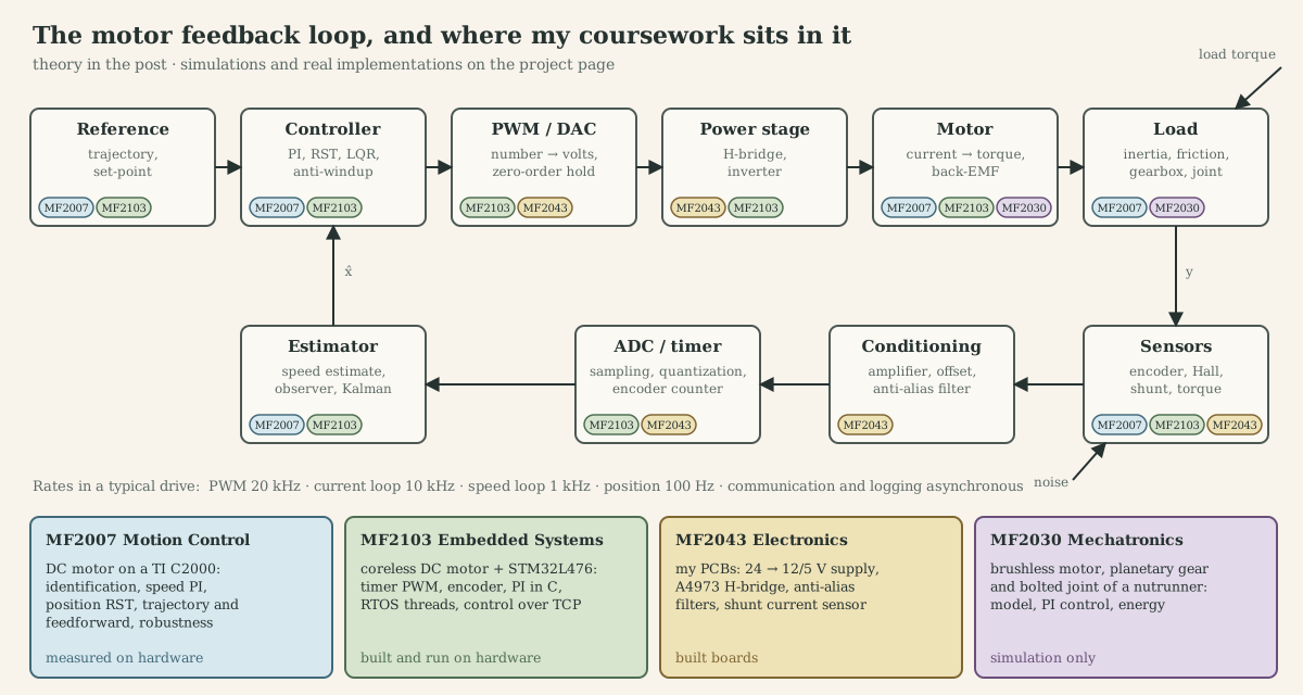
| Loop block | Question | Part |
|---|---|---|
| Actuator | Which physical effect converts energy into force or torque, and what limits it? | A (actuators), B (electromagnetics), C (machine types) |
| Plant model | Which equations describe the motor and its load? | D (DC motor), I (BLDC/PMSM) |
| Sensors | What is measured, how well and how fast? | E (encoders, Hall, resolvers, current, torque) |
| Converters | How does a signal cross between the analog and the digital world? | F (sampling, aliasing, cut-off, ADC, DAC, PWM) |
| Controller | What do we feed back, at which rate, and what happens at the limits? | G (PID, cascades, servo, LQR, discretization, anti-windup) |
| Estimator | How do we get states we cannot measure, from data we do not fully trust? | H (observers, Kalman, complementary filters, PLLs, sensorless) |
| Power stage | Which circuit turns a duty cycle into winding current? | J (MOSFETs, H-bridges, inverters, current paths) |
| Firmware | Which code runs on which core, and when? | K (embedded C), L (concurrency), M (real time), N (RTOS and Zephyr) |
| The whole loop | How do we debug it and size it? | O (debugging), P (integrated chain), Q (worked example) |
Each part moves through five levels and says which one it is on:
| Level | Question | Typical objects |
|---|---|---|
| Physics | What converts energy, and what limits it? | fields, forces, flux, pressure, heat |
| Model | Which equations capture the behaviour we can control? | ODEs, transfer functions, state space, maps |
| Control and estimation | What do we feed back, how fast, with what guarantee, and how do we estimate it? | P/PI/PID, state feedback, observers, Kalman filters |
| Electronics | Which circuit turns a number into volts and amps, and back? | MOSFETs, bridges, sensors, amplifiers, filters, ADCs |
| Embedded | Which code, on which core, at which moment? | registers, ISRs, threads, timers, fixed point |
The examples come from the hardware and models I worked with; the project page tags every parameter as built, measured, modelled, datasheet, assumed or unknown:
- MF2007 rig (real hardware): a small DC motor with a 3600-pulse encoder on a TI C2000 LaunchPad (identified $J$, friction, speed and position control).
- MF2103 platform (real hardware): a coreless DC motor with encoder, a dual half-bridge shield and an STM32L476 Nucleo board running my speed-control firmware (super-loop, RTOS and TCP versions).
- MF2043 boards (built): a 24 V → 12 V/5 V supply, an A4973 H-bridge, passive and active anti-alias filters and a shunt current sensor.
- MF2030 model (simulation): a Faulhaber BX4 brushless motor with a planetary gearbox and a bolted joint, from an Atlas Copco nutrunner. It serves as the application example in Part Q.
Conventions
| Symbol | Meaning | Unit |
|---|---|---|
| $V$, $v$ | applied (terminal) voltage, average over a PWM period unless stated | V |
| $i$ | winding current | A |
| $R$, $L$ | winding resistance and inductance (line-to-line for three-phase datasheets) | Ω, H |
| $k_t$, $k_e$ | torque constant, back-EMF constant; equal in SI units | N·m/A, V·s/rad |
| $\omega$, $\theta$ | motor (mechanical) speed and angle | rad/s, rad |
| $\theta_e = p\,\theta_m$ | electrical angle, $p$ pole pairs | rad |
| $J$, $b$ | inertia, viscous friction | kg·m², N·m·s/rad |
| $n$, $\eta$ | gear ratio (motor turns per output turn), gear efficiency | –, – |
| $N_{\text{cpr}}$ | encoder counts per revolution (after quadrature decoding) | – |
| $T_s$, $f_s$ | sampling period and rate | s, Hz |
| $f_c$, $\omega_c$ | filter cut-off frequency, or loop crossover frequency (context says which) | Hz, rad/s |
| $f_{\text{PWM}}$, $D$ | PWM frequency and duty cycle | Hz, – |
Speeds in rpm are converted with $\omega\,[\text{rad/s}] = \text{rpm}\cdot 2\pi/60$. “Phase-phase” or “terminal” resistance in BLDC datasheets is between two motor leads, which is what a six-step drive sees.
Contents
- Part A. Actuators: physics, models, selection
- Part B. Electromagnetic foundations
- Part C. Electric machine taxonomy
- Part D. The DC motor as the first complete model
- Part E. Sensors: what the loop actually sees
- Part F. The signal chain: sampling, filters, ADC, DAC and PWM
- Part G. Feedback control: continuous and discrete
- Part H. Estimation and sensor fusion
- Part I. BLDC and PMSM modelling and control
- Part J. Power electronics between MCU and motor
- Part K. Embedded foundations: below the abstraction
- Part L. Concurrency and synchronization
- Part M. Real-time systems and control timing
- Part N. RTOS in practice: CMSIS-RTOS and Zephyr
- Part O. Debugging electromechanical systems
- Part P. The integrated chain
- Part Q. Worked example: sizing a drive for a tightening application
- References and reading guide
Related posts: Control Theory Basics · Modern, Multivariable, and Networked Control · Adaptive, Optimal, Robust, and Learning Control · Signals and Systems · Electronics · C++ · Numerical Linear Algebra and Optimization · Lie Groups for Robotics · Distributed Systems.
Part A. Actuators: physics, models, selection
A.1 An actuator is a controlled energy converter
An actuator takes power from a source, modulates it according to a low-power command, converts it to mechanical form and delivers it through a transmission to a load. Writing the chain explicitly prevents the most common selection error: comparing actuators by their converter alone (a cylinder, a motor) and forgetting the modulator and source that must come with it.
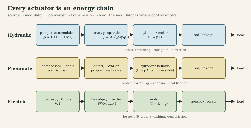
Power variables. Each stage carries power as a product of an effort and a flow:
| Domain | Effort | Flow | Power | Storage (capacitive / inductive) |
|---|---|---|---|---|
| Electrical | voltage $v$ | current $i$ | $v\,i$ | capacitor / inductor |
| Translational | force $F$ | velocity $\dot x$ | $F\dot x$ | spring / mass |
| Rotational | torque $\tau$ | speed $\omega$ | $\tau\omega$ | torsion spring / inertia |
| Hydraulic | pressure $p$ | volume flow $Q$ | $pQ$ | compressibility / fluid inertance |
| Thermal (pseudo) | temperature $T$ | heat flow $\dot Q$ | – | heat capacity |
A lossless transducer couples two domains with one of two structures. A transformer scales effort and flow inversely (gear: $\tau_{\text{out}} = n\tau_{\text{in}}$, $\omega_{\text{out}}=\omega_{\text{in}}/n$; piston: $F = pA$, $Q = A\dot x$). A gyrator crosses them (motor: $\tau = k_t i$ and $e = k_e\omega$, so current maps to torque and speed maps to voltage). This is why an electric motor behaves like a gyrator: a voltage source at the terminals looks like a speed source at the shaft, and a current source looks like a torque source. That one fact shapes the whole control architecture in Parts D-F (current loop = torque control).
Figures of merit and what sets them:
| Property | Definition | What limits it |
|---|---|---|
| Force/torque density | max force per mass or volume | pressure (fluid), magnetic shear stress and current density (electric) |
| Power density | max power per mass | force density × achievable speed; cooling |
| Efficiency | output/input power | throttling, $I^2R$, iron loss, friction, compressor efficiency |
| Bandwidth | frequency up to which the actuator follows a command | modulator speed, compliance (fluid), inductance and current limit (electric), inertia |
| Stiffness | $\partial F/\partial x$ seen by a load disturbance | fluid bulk modulus, feedback gain, transmission compliance |
| Controllability | how directly the command maps to force or position | linearity, hysteresis, dead band, friction |
Typical orders of magnitude: hydraulic actuators reach working pressures of 100-300 bar, so a 25 mm bore produces 5-15 kN; magnetic shear stress in electric machines is a few to a few tens of kPa, so electric actuators need gearing or screws to reach the same forces; pneumatic systems run at 6-8 bar and are soft and cheap.
A.2 Mechanical transmission: the actuator’s impedance matcher
A motor produces small torque at high speed; a bolt needs large torque at low speed. The transmission matches them.
Ideal gear. With ratio $n$ (motor turns per output turn):
\[\omega_{\text{out}}=\frac{\omega_m}{n},\qquad \tau_{\text{out}}=\eta\,n\,\tau_m\ \ (\text{driving}),\qquad \tau_{\text{out}}=\frac{n\,\tau_m}{\eta}\ \ (\text{back-driven}).\]The efficiency $\eta$ appears differently in the two power-flow directions; a low-efficiency worm or lead screw ($\eta<0.5$) is self-locking because back-driving would need negative friction.
Reflected inertia and load. Write Newton’s law on the motor shaft for a motor inertia $J_m$ and a load inertia $J_L$ on the output:
\[\Big(J_m+\frac{J_L}{\eta n^2}\Big)\dot\omega_m=\tau_m-\frac{\tau_L}{\eta n}-b_m\omega_m .\]The load inertia is divided by $n^2$ and the load torque by $n$. This is the most important equation of the transmission: the controller sees the load through the gearbox, so a large ratio makes the plant almost independent of the load (good for robustness) but makes the motor’s own inertia dominate (bad for acceleration and for sensing the load through motor current).
Ratio for best acceleration. For a pure inertial load, the load acceleration $\ddot\theta_L=\tau_m n/(J_m n^2+J_L)$ is maximized at
\[n^\ast=\sqrt{J_L/J_m},\]where the reflected load inertia equals the motor inertia (“inertia matching”). Most practical drives use $n>n^\ast$ because speed limits, torque limits and robustness matter more.
Nonidealities that enter the model:
- Compliance. Shafts, gear teeth and couplings are springs. Splitting the system into motor side and load side connected by stiffness $K$ and damping $d$ gives a two-mass model with an anti-resonance (load side vibrates, motor side still) and a resonance (both move in opposition). With motor-side sensing, the controller sees the anti-resonance zero first; this limits the bandwidth of the speed loop. The MF2030 nutrunner model is exactly such a model (A.2 case-study hook).
- Backlash. A dead zone of angle $\Delta$: no torque is transmitted until the gap closes. It creates limit cycles under integral control and impact torques at reversals.
- Friction. Coulomb ($F_c\,\mathrm{sign}(\omega)$), viscous ($b\omega$) and static (stiction) components; the MF2007 identification found that adding Coulomb friction to the linear model fixed the low-voltage step responses (Part D.7).
- Efficiency vs load. Gear efficiency drops at light load (fixed churning losses), so $\eta$ quoted at rated torque overestimates low-torque efficiency.
Common transmissions. Spur and planetary gears (planetary: coaxial, high torque density, ratios 3-10 per stage, $\eta\approx 0.9-0.97$ per stage); harmonic drives (ratios 50-160 in one stage, zero backlash, compliant); belts (cheap, compliant, quiet); lead and ball screws (rotary to linear, $F=2\pi\eta\tau/p$ for lead $p$; ball screws have $\eta\approx0.9$, lead screws 0.2-0.6); bevel or spiral-bevel angle gears (change axis, as in the nutrunner’s angle head).
Case-study hook. The nutrunner has two planetary stages (chosen as $9\times9=81$ in the MF2030 report) and a spiral-bevel angle head. The model lumps input-side inertia $J_i=6.2\cdot10^{-6}$ kg·m² (motor rotor $6.0\cdot10^{-6}$ plus shaft and planet carriers) and output-side inertia $J_o=5.6\cdot10^{-6}$ kg·m², joined by a torsional stiffness $K_t=739$ N·m/rad and damping $d_t=1.5$ N·m·s/rad. Part Q revisits whether 81 is the right ratio.
A.3 Thermal and combustion actuation
Heat engines convert chemical energy to work through a thermodynamic cycle; their efficiency is bounded by Carnot and in practice reaches 25-40 % for automotive engines over a narrow speed-torque band, which is why hybrid powertrains add an electric machine that covers transients and recovers braking energy (MF2007 C2). As servo actuators, combustion engines are slow (torque responds within cycles, not microseconds) and are controlled through fuel, air and ignition timing rather than directly.
Thermal actuators (bimetal strips, wax pellets in thermostats, shape-memory alloys) produce motion from thermal expansion or phase change. Their bandwidth is set by a thermal time constant $\tau_{\text{th}}=R_{\text{th}}C_{\text{th}}$ of seconds, they are strongly hysteretic, and their efficiency is a few percent; they are used where silence, simplicity or force density at small scale matters more than speed. Thermal time constants matter for every actuator, though: the winding temperature of a motor obeys the same first-order model and sets its continuous rating (Part B.6).
A.4 Hydraulic actuation
Working principle. A pump converts shaft power into pressurized flow; a valve meters that flow; a cylinder or hydraulic motor converts pressure into force or torque. Because oil is nearly incompressible and pressures are high, hydraulics offers the highest force density and a stiff, fast actuator, at the cost of leakage, noise, fire risk and low efficiency when throttling.
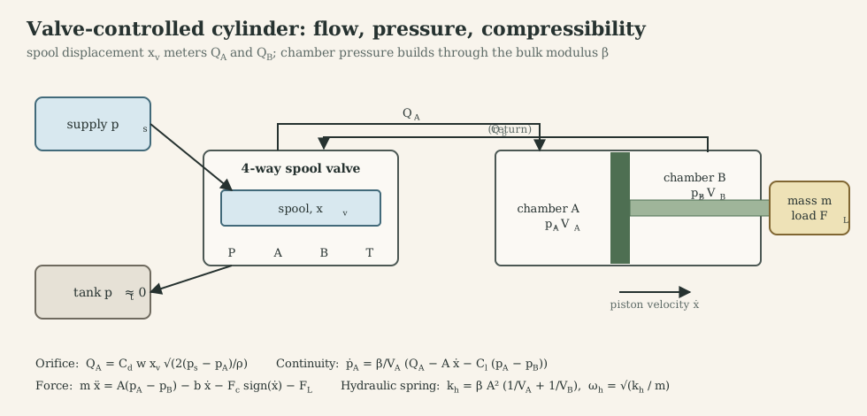
Orifice flow. Flow through a sharp-edged valve port of area $A_v=w\,x_v$ (port width $w$, spool displacement $x_v$) follows Bernoulli with a discharge coefficient $C_d\approx0.6$:
\[Q = C_d\,w\,x_v\sqrt{\frac{2\,\Delta p}{\rho}} .\]It is nonlinear in both $x_v$ (through sign changes) and $\Delta p$. Linearizing around an operating point gives the valve coefficients
\[\Delta Q = K_q\,\Delta x_v - K_c\,\Delta p_L,\qquad K_q=\frac{\partial Q}{\partial x_v},\quad K_c=-\frac{\partial Q}{\partial p_L},\]with $K_q$ the flow gain (largest at no load) and $K_c$ the flow-pressure coefficient (zero at the null of an ideal critically-lapped valve, which is exactly where damping is most needed).
Chamber continuity. Oil is slightly compressible with bulk modulus $\beta$ ($\approx1.4$ GPa for pure oil, often 0.7-1 GPa effective with entrained air and hose compliance). Mass conservation in chamber A of volume $V_A$:
\[\frac{V_A}{\beta}\,\dot p_A = Q_A - A\,\dot x - C_{l}\,(p_A-p_B),\]with $C_l$ the internal leakage coefficient. Force balance on piston and load:
\[m\ddot x = A(p_A-p_B) - b\dot x - F_c\,\mathrm{sign}(\dot x) - F_L .\]The hydraulic spring. Combining both chambers, the trapped oil acts as a spring
\[k_h = \beta A^2\Big(\frac1{V_A}+\frac1{V_B}\Big),\qquad \omega_h=\sqrt{k_h/m}.\]With a 25 mm bore ($A=5\ \text{cm}^2$), 50 cm³ per chamber, $\beta=1.4$ GPa and $m=20$ kg: $k_h=1.4\cdot10^{7}$ N/m and $\omega_h\approx 840$ rad/s (130 Hz). The linearized valve-cylinder transfer function from spool to velocity is a lightly damped second-order system at $\omega_h$, with damping ratio set by $K_c$ and leakage, typically only 0.05-0.2. This lightly damped hydraulic resonance, not the valve, usually limits closed-loop bandwidth: a proportional position loop must keep its crossover well below $\omega_h$ (a rule of thumb is $K_v<0.2-0.3\,\omega_h$ for the velocity gain).
Losses. Every throttling edge dissipates $Q\,\Delta p$; a valve-controlled system at constant supply pressure wastes the difference between supply and load pressure, which is why load-sensing pumps and pump-controlled (displacement-controlled) actuators exist.
Sensors and control. Position (LVDT, magnetostrictive), chamber pressures, spool position (internal valve loop). Control laws: proportional position control with velocity feedback; pressure feedback to add damping (it effectively increases $K_c$); feedforward of flow; robust or adaptive control for varying load and bulk modulus.
Case-study hook (MF2007 Workshop B). My group designed a velocity controller for a valve-controlled cylinder and tested it against an external force, a change of load mass and sensor noise. The observation that faster observer poles improved disturbance rejection but transmitted more sensor noise is the hydraulic version of the $S+T=1$ trade-off in Part G.8.
A.5 Pneumatic actuation
Air replaces oil: cheap, clean, safe, and $\beta$ is no longer large. For an ideal gas undergoing a fast (adiabatic) process the effective bulk modulus is $\beta=\kappa\,p$ with $\kappa=1.4$; at 6 bar absolute, $\beta\approx0.84$ MPa, about 1700 times smaller than oil. The same cylinder as above then has $k\approx8.4\cdot10^{3}$ N/m and $\omega\approx20$ rad/s (3 Hz). Pneumatic actuators are soft, which is excellent for compliant contact and bad for precise position control.
Flow. Compressible flow through an orifice is choked (sonic) when the downstream-to-upstream pressure ratio falls below about 0.53; the mass flow then depends only on upstream pressure. In the unchoked region it depends on both pressures. Chamber pressure dynamics:
\[\dot p=\frac{\kappa R T}{V}\dot m_{\text{in}}-\frac{\kappa\,p}{V}A\dot x .\]Nonlinearities. Choked/unchoked switching, large seal friction with stick-slip, temperature dependence, long transport delays in hoses. Control. Most pneumatic axes are end-to-end (on/off valves, mechanical stops); servo-pneumatics uses proportional valves or fast PWM on/off valves with pressure feedback and friction compensation. The DeLaval milking-valve project used a vacuum-actuated pinch valve under cascade PID: the same chamber-pressure physics with sub-atmospheric pressure.
A.6 Electromagnetic and other electrical actuators
- Solenoid (reluctance actuator). A plunger is pulled into a coil to shorten the air gap; force $F=\tfrac12 i^2\,\mathrm{d}L/\mathrm{d}x$ grows strongly as the gap closes (Part B.3). Single-acting (spring return), short stroke, very nonlinear. My MF2043 lab 2 drove a 40 mH, 13 Ω solenoid from 24 V with a MOSFET: the electrical time constant $L/R\approx3$ ms limits how fast force builds, and the freewheel diode placement decides how fast it decays (Part J.3).
- Voice coil (Lorentz actuator). A coil in a permanent-magnet gap: $F=B\,l\,i$, linear in current, no cogging, bandwidths of kHz; short stroke. MF2030 lecture 9 models it as a linear electrical actuator.
- Piezoelectric. Strain from electric field: nanometre resolution, kHz-MHz bandwidth, micrometre stroke, capacitive load needing current-controlled drive.
- Electrostatic. Force from charge on electrodes; dominant in MEMS.
- Rotary electric motors. The rest of this post.
A.7 Comparison and selection
| Hydraulic | Pneumatic | Electric (motor + gear/screw) | |
|---|---|---|---|
| Force/torque density | highest | low | medium (needs transmission) |
| Stiffness (open loop) | high (oil) | low (air) | set by transmission and control |
| Bandwidth | high, limited by $\omega_h$ | low | highest at the current loop |
| Efficiency | low when throttling | low (compressor) | high (80-95 % motor) |
| Precision | good with servo valve | poor without effort | excellent |
| Holding force | needs pressure or lock valve | needs pressure | needs current or brake |
| Overload behaviour | relief valve, graceful | compliant, graceful | current limit, thermal |
| Infrastructure | pump, tank, hoses | compressor, air lines | battery or DC bus |
| Cleanliness, noise | leaks, noisy | clean, exhaust noise | clean, quiet |
Selection procedure: (1) write the motion profile (force/torque and speed versus time); (2) compute peak and RMS force and power; (3) list constraints (mass, envelope, energy source, environment, safety); (4) choose the family; (5) size converter and transmission against peak and RMS demand and thermal limits; (6) check bandwidth and stiffness against the control requirements.
Case-study hook. For a hand-held tightening tool the energy source is a battery, the duty is intermittent, accuracy of final torque matters (traceable to standards for safety-critical joints), and the tool must be quiet and light: a brushless motor with planetary gearing and a torque transducer is the natural answer, which is what the Tensor STB uses.
What to remember
- Actuator = source → modulator → converter → transmission → load; compare whole chains.
- The motor is a gyrator: current ↔ torque, speed ↔ voltage. Current control is torque control.
- Gearing divides load inertia by $n^2$ and load torque by $n$; compliance and backlash enter the loop.
- Hydraulic bandwidth is limited by the oil spring $\omega_h=\sqrt{\beta A^2(1/V_A+1/V_B)/m}$; pneumatics is ~40× softer at equal geometry.
Part B. Electromagnetic foundations
Motor names (DC, BLDC, PMSM, induction) describe how a machine arranges a small number of physical effects. This part builds those effects in order: current makes field, field and current make force, motion makes voltage, and geometry turns force into continuous torque.
B.1 From current to field to force
Ampère’s law. A current $i$ through $N$ turns produces a magnetomotive force $\mathcal{F}=N i$ around any closed path linking the turns: $\oint \mathbf H\cdot d\mathbf l = N i$. In a material, $\mathbf B=\mu_0\mu_r\mathbf H$; iron has $\mu_r$ in the thousands until it saturates at roughly 1.5-2 T.
Lorentz force. A conductor of length $l$ carrying current $i$ in a flux density $B$ perpendicular to it feels
\[\mathbf F = i\,\mathbf l\times\mathbf B,\qquad |F| = B\,l\,i .\]At radius $r$ the force gives a torque $\tau = r B l i$. A rectangular coil of $N$ turns with two active sides gives $\tau = 2NrBl\,i\cos\alpha$, where $\alpha$ is the angle between the coil plane and the field: maximum when the coil sides cross the field at right angles, zero when they are aligned. A single coil in a fixed field produces a torque that reverses every half revolution. Everything about commutation follows from this sentence.
B.2 Magnetic circuits, reluctance and inductance
Flux $\Phi=\int\mathbf B\cdot d\mathbf A$ is continuous around a closed iron path, like current in a circuit. Each segment of length $l$ and cross-section $A$ has a reluctance $\mathcal R=l/(\mu A)$, and
\[\Phi=\frac{N i}{\sum\mathcal R},\qquad \lambda=N\Phi,\qquad L=\frac{\lambda}{i}=\frac{N^2}{\sum\mathcal R}.\]Because $\mu_r\gg1$ in iron, a small air gap dominates the total reluctance: $\mathcal R_{\text{gap}}=g/(\mu_0A)$.
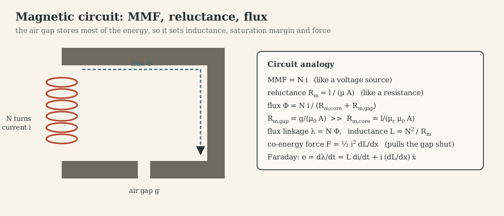
Worked numbers. $N=100$ turns, $i=1$ A, gap $g=1$ mm, pole area $A=1$ cm², iron reluctance neglected: $B=\mu_0Ni/g=0.126$ T, $L=\mu_0N^2A/g=1.26$ mH, and the force pulling the gap closed is $F=B^2A/(2\mu_0)=0.63$ N. Halve the gap and $B$ doubles, $L$ doubles and the force quadruples: reluctance actuators are strongly nonlinear in position.
Saturation. Once the iron saturates, $\mu_r$ collapses, $L$ drops and extra current produces little extra flux. In motors, saturation flattens the torque-current curve at high current (the datasheet $k_t$ is a small-signal value) and makes $L$ current-dependent, which matters for current-loop tuning.
B.3 Energy, co-energy and force
For a lossless electromechanical device with flux linkage $\lambda(i,x)$, energy input is $v\,i\,dt=i\,d\lambda$. The co-energy \(W'(i,x)=\int_0^i\lambda(i',x)\,di'\) gives the force at constant current:
\[F=\frac{\partial W'}{\partial x}\Big|_{i},\qquad\text{linear magnetics: } W'=\tfrac12L(x)i^2\ \Rightarrow\ F=\tfrac12 i^2\frac{dL}{dx}.\]Two mechanisms appear: reluctance force (the iron moves to increase $L$, the solenoid and the switched-reluctance motor) and alignment force between a current and a permanent magnet (the Lorentz picture, the DC and PM synchronous machines). Rotary machines use the angular form \(\tau=\partial W'/\partial\theta\).
B.4 Faraday’s law and back-EMF
A changing flux linkage induces a voltage:
\[e=\frac{d\lambda}{dt}=L\frac{di}{dt}+\frac{\partial\lambda}{\partial x}\dot x .\]The first term is the self-induced voltage of the winding; the second is the motional (back) EMF. For a coil moving through a permanent-magnet field, $\partial\lambda/\partial\theta$ is a constant $k_e$ (for a DC machine, averaged by the commutator), so $e=k_e\omega$.
Why $k_t=k_e$. Electrical power converted to mechanical is $e\,i$; mechanical power is $\tau\omega$. Conservation of energy gives $k_e\omega\,i=k_t i\,\omega$, so in SI units
\[k_t\,[\text{N·m/A}] = k_e\,[\text{V·s/rad}].\]Datasheets use mixed units. The Faulhaber 3268 BX4 lists $k_e=4.555$ mV/rpm and $k_t=43.5$ mN·m/A; converting, $4.555\cdot10^{-3}\cdot60/(2\pi)=0.0435$ V·s/rad, equal to 0.0435 N·m/A. The “speed constant” 220 rpm/V is simply $1/k_e$. Checking this equality is the first sanity test of any motor parameter set.
B.5 From coil to machine: poles, commutation and the rotating field
A practical machine has a stator (stationary) and a rotor (rotating), separated by a small air gap through which the useful flux crosses radially. One side carries the field (permanent magnets or a field winding), the other carries the armature winding whose current is controlled.
Pole pairs. A machine with $p$ pole pairs repeats its magnetic pattern $p$ times per revolution, so electrical quantities cycle $p$ times per mechanical turn:
\[\theta_e=p\,\theta_m,\qquad \omega_e=p\,\omega_m,\qquad f_e=\frac{p\,\text{rpm}}{60}.\]MF2030 calls the pole number “a gear between electrical and mechanical angle”. The Faulhaber BX4 has $p=2$: at 5500 rpm the phase currents alternate at 183 Hz, and a six-step drive commutates 1100 times per second.
Commutation. Because the torque of a coil reverses every half electrical period (B.1), the current must be reversed in step with rotor position:
- Mechanical commutation: brushes sliding on a segmented commutator switch the rotor coils (brushed DC motor). The commutator is a rotary switch synchronized by construction.
- Electronic commutation: the windings are on the stator, a position sensor (Hall sensors, encoder) or estimator reports rotor angle, and transistors switch the currents (BLDC, PMSM).
Rotating field. Three windings displaced by 120° electrical and fed with balanced sinusoidal currents $i_a=I\cos\theta_e$, $i_b=I\cos(\theta_e-2\pi/3)$, $i_c=I\cos(\theta_e+2\pi/3)$ produce a magnetic field of constant magnitude $\tfrac32 I$ (in winding units) that rotates at $\omega_e$. A permanent-magnet rotor locks to it (synchronous machine); a conducting rotor slips behind it and has current induced (induction machine). MF2030’s two-winding pictures make the same point with $\alpha$ and $\beta$ windings: rotating at constant speed gives AC winding currents, standing still gives DC.
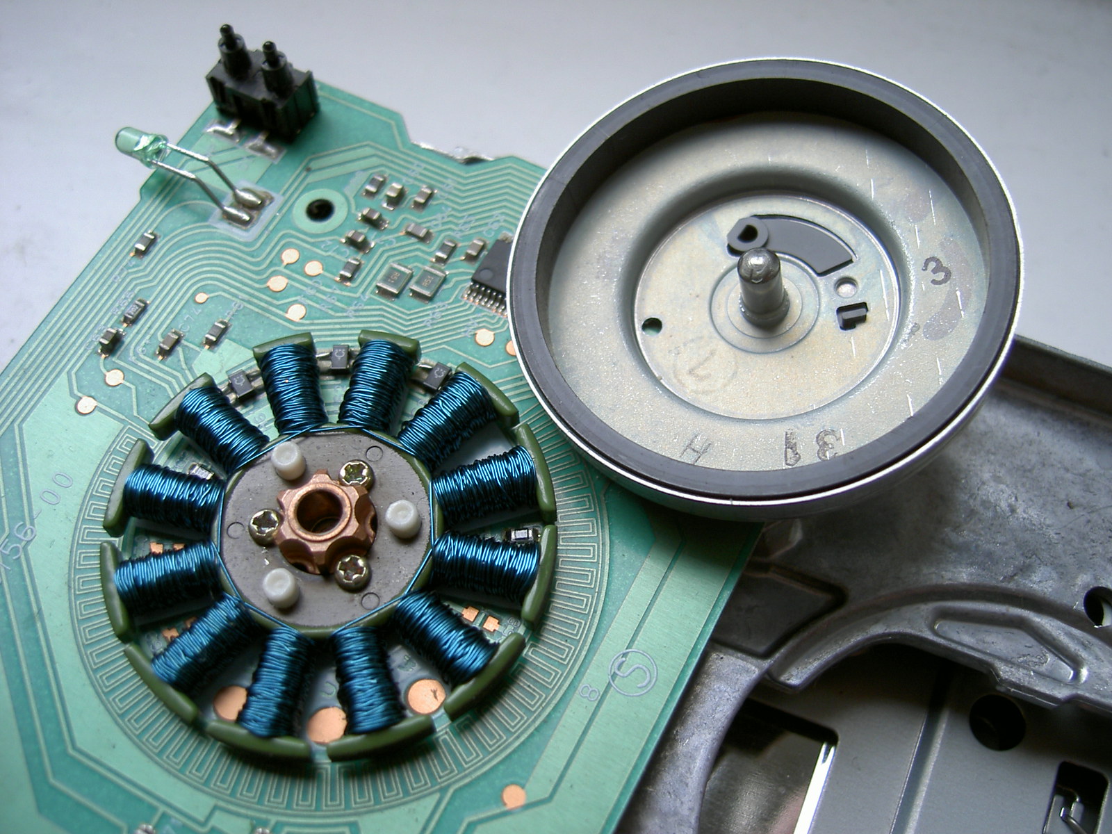
How geometry produces useful torque. The tangential force per unit air-gap area, the air-gap shear stress $\sigma$, is the product of the gap flux density and the linear current density of the winding. Torque scales as
\[\tau = \sigma\cdot(2\pi r l)\cdot r = 2\,\sigma\,V_{\text{rotor}} ,\]so torque is proportional to rotor volume, not to speed. Shear stress is limited by flux density (iron saturation) and current density (heating), roughly a few kPa for small air-cooled motors and up to tens of kPa for large or liquid-cooled machines. This is why small motors are fast and geared: power is torque times speed, and torque per volume is capped.
B.6 Non-idealities: ripple, cogging, losses and heat
- Torque ripple comes from imperfect commutation (BLDC six-step), non-sinusoidal back-EMF, current ripple from PWM, and current-sensor offsets (which produce ripple at the electrical frequency in FOC).
- Cogging torque is a reluctance torque between magnets and stator teeth that exists with zero current. Slotless and coreless designs (like the Assun coreless motor in MF2103) have essentially none, at the price of a larger magnetic gap and lower inductance.
- Losses: copper loss $I^2R$ (with $R$ rising about 0.39 %/K in copper, so a winding at 125 °C has about 40 % more resistance than at 22 °C); iron loss from hysteresis and eddy currents, growing with electrical frequency; friction and windage; PWM ripple losses in the winding and the magnets.
- Thermal model. A two-node model is standard: winding to housing $R_{th1}$ with time constant $\tau_{w1}$, housing to ambient $R_{th2}$ with $\tau_{w2}$. For the BX4: $R_{th1}=1.9$ K/W, $R_{th2}=9.6$ K/W, $\tau_{w1}=17$ s, $\tau_{w2}=1060$ s. The fast winding constant permits short overloads; the slow housing constant sets the continuous rating (1.41 A thermally insulated, 2.59 A when $R_{th2}$ is reduced 55 % by mounting to a heat sink).
B.7 Torque-speed behaviour and operating regions
For a permanent-magnet DC machine at constant voltage $V$ (Part D derives this properly):
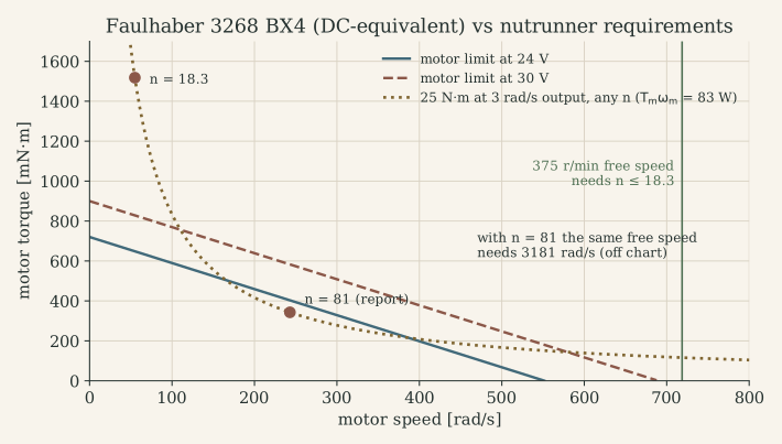
\[\tau = \frac{k_t}{R}\big(V-k_e\omega\big):\quad \tau_{\text{stall}}=\frac{k_t V}{R},\quad \omega_0=\frac{V}{k_e},\quad P_{\max}=\frac{V^2}{4R}\ \text{at}\ \omega_0/2 .\]For the BX4 at 24 V: $\tau_{\text{stall}}=0.72$ N·m, $\omega_0=552$ rad/s (5270 rpm, the datasheet gives 5500), $P_{\max}=99$ W, while the thermally continuous rating is about 33 W. The torque-speed plane therefore has three boundaries:
- Current (torque) limit: set by the drive’s current limit and short-term thermal capacity. Below it, any torque can be produced at any speed: the constant-torque region.
- Voltage limit: the line above, where back-EMF plus $IR$ drop uses up the available voltage.
- Thermal (RMS) limit: the continuous operating area, much smaller than the peak area.
In PM synchronous machines, injecting negative $i_d$ (Part I.7) weakens the effective field, lowers back-EMF and extends speed beyond the base speed at roughly constant power: the constant-power region. Induction machines get the same effect by reducing flux.
Common misconceptions
- “Higher voltage gives more torque.” At stall, yes; but torque is set by current. Voltage sets the speed at which a given torque can still be reached.
- “k_t and k_e are different motor properties.” In SI they are the same number; a datasheet that disagrees is using different units or RMS conventions (three-phase datasheets often quote $k_{t,\text{rms}}$, which differs by $\sqrt2$ or $\sqrt3$ factors).
- “Peak power is the motor rating.” Peak power is at half no-load speed with 50 % efficiency; the continuous rating is thermal and usually far lower.
What to remember
- Current → field (Ampère, reluctance); field + current → force (Lorentz, co-energy); motion → voltage (Faraday).
- $k_t=k_e$ in SI units; convert datasheets carefully.
- $\theta_e=p\theta_m$; commutation reverses current in step with position.
- Torque scales with rotor volume; speed is cheap, torque is expensive; heat sets continuous ratings.
Part C. Electric machine taxonomy
Four machine types cover almost all servo and tool drives. Each one is described by the same twelve questions, first in prose with the defining equations, then in one comparison table.
C.1 Brushed DC motor
Construction. Permanent magnets (or a field winding) on the stator; the armature winding on the rotor, connected through a commutator (copper segments) and brushes (graphite or precious metal). Coreless (ironless, “bell”) rotors such as the Assun AM-CL1643MB-1210 in MF2103 wind the coil as a self-supporting cylinder rotating in the gap: no iron in the rotor, so no cogging, very low inertia (3.11 g·cm²) and very low inductance (0.21 mH).
Operating principle and commutation. Brushes feed current into whichever rotor coils are passing under the magnet poles; the commutator reverses each coil’s current as it crosses the neutral zone, so the torque from all active conductors always adds (B.1). Commutation is mechanical and automatic: the motor runs from a DC source without any electronics.
Electrical and mechanical model.
\[V = R i + L\frac{di}{dt} + k_e\omega,\qquad J\dot\omega = k_t i - b\omega - \tau_L .\](Brush contact drop, a nearly constant 0.2-2 V, and commutation ripple are ignored.) Torque is proportional to current, independent of position: the simplest possible torque actuator.
Sensing and drive. Optional encoder or tachometer for speed/position; current through a shunt. Drive: one transistor for unidirectional speed control, an H-bridge for four-quadrant operation (Part J).
Pros / cons. Simple, cheap, linear, easy to control. Brushes wear, spark (EMI), limit speed, and the rotor heat must leave through the air gap, which limits continuous torque.
C.2 Induction (asynchronous) motor
Construction. Three-phase stator winding; rotor with a short-circuited cage (aluminium or copper bars and end rings), no magnets, no brushes.
Principle. The stator’s rotating field (B.5) at synchronous speed $\omega_s=\omega_e/p$ sweeps past the rotor bars. If the rotor turns slower, at $\omega_m$, the relative motion induces rotor currents whose interaction with the field produces torque. The slip
\[s=\frac{\omega_s-\omega_m}{\omega_s}\]must be non-zero for torque to exist: the machine is “asynchronous”.
Equivalent circuit (per phase). Stator resistance and leakage $R_s$, $L_{ls}$; magnetizing inductance $L_m$; rotor leakage \(L_{lr}'\) and a rotor resistance that appears as \(R_r'/s\). The power crossing the air gap is \(P_{ag}=3I_r'^2R_r'/s\), and
\[\tau=\frac{p\,P_{ag}}{\omega_e}=\frac{3p}{\omega_e}I_r'^2\frac{R_r'}{s}.\]Torque rises roughly linearly with slip, reaches a breakdown maximum, and falls; the useful region is at small slip. MF2030 lists the no-load test (measures the magnetizing branch, or $k_e$ for a PM machine) and the short-circuit or locked-rotor test (measures the series impedance) used to identify such circuits.
Control. V/f (scalar) control for pumps and fans; field-oriented control (rotor-flux orientation, needs a flux estimate and slip calculation); direct torque control. Pros / cons. Robust, cheap, brushless, field can be weakened easily; lower efficiency and torque density than PM machines, rotor losses heat the rotor, and precise control needs a model of rotor time constant.
C.3 BLDC motor (trapezoidal PM machine)
Construction. Three-phase stator winding (usually star-connected), permanent-magnet rotor (inner rotor or outrunner, as in the floppy spindle photo above), and three Hall sensors placed 120° (or 60°) electrical apart. The Faulhaber 3268 BX4 is this type: 4 poles ($p=2$), integrated Hall sensors, optional encoder.
Principle and commutation. Concentrated windings give a trapezoidal back-EMF with flat tops 120° electrical wide. If constant current flows in the two phases whose back-EMF is in a flat region, power $e_a i_a+e_b i_b+e_c i_c$ and therefore torque is constant. The Hall sensors divide each electrical period into six sectors; in each sector one phase is driven high, one low, one floats: six-step (120°) commutation (Part I.2).
Model. For each phase,
\[v_x = R\,i_x + L\frac{di_x}{dt} + e_x(\theta_e) + v_n,\qquad x\in\lbrace a,b,c\rbrace ,\]with $L$ the self minus mutual inductance and $v_n$ the star-point voltage; torque $\tau=(e_ai_a+e_bi_b+e_ci_c)/\omega_m$. Under six-step drive two phases are in series and the DC side sees
\[V_{dc}=R_{ll}\,I+L_{ll}\frac{dI}{dt}+k_{e}\,\omega ,\]with line-to-line $R_{ll}=2R$, $L_{ll}=2L$ and the line-to-line back-EMF constant. This is exactly a DC motor model, which is why datasheets quote “terminal resistance, phase-phase” and why the MF2030 report could model the BX4 as a DC motor. The equivalence holds for torque production on average; it hides commutation ripple and the 60° steps of current direction.
Pros / cons. No brushes, the heat is in the stator (easy to cool), high speed and power density, simple six-step control with three Hall sensors. Torque ripple at commutation (5-15 % is common), audible noise, and the six-step current waveform is not ideal for smooth low-speed servo motion.
C.4 PMSM (sinusoidal PM machine)
Construction. Like a BLDC motor but with distributed (sinusoidal) windings and/or shaped magnets so that the back-EMF is sinusoidal. Magnets may be surface-mounted (SPM, $L_d\approx L_q$) or interior (IPM, $L_q>L_d$, adds reluctance torque).
Principle. Sinusoidal phase currents in phase with the back-EMF give constant torque without commutation ripple. Control requires a continuous rotor angle (encoder, resolver, or an observer), not just six Hall sectors.
Model. In rotor coordinates (Part I.4):
\[v_d=Ri_d+L_d\frac{di_d}{dt}-\omega_eL_qi_q,\quad v_q=Ri_q+L_q\frac{di_q}{dt}+\omega_eL_di_d+\omega_e\psi_m,\quad \tau=\tfrac32p\big[\psi_mi_q+(L_d-L_q)i_di_q\big].\]Control. Field-oriented control with SVPWM; field weakening above base speed; MTPA for IPMs. Pros / cons. Smoothest torque, highest efficiency and torque density; needs a precise position sensor and the most complex control and electronics.
C.5 Servo motor versus servo system
“Servo” is a property of a closed-loop system, not of a winding. A servo system has five parts:
- a motor (DC, BLDC or PMSM),
- a feedback sensor (encoder, resolver, Hall sensors, potentiometer, torque transducer),
- a drive (power stage plus current loop, usually also speed and position loops),
- a motion controller (trajectory generation, outer loops, sequencing),
- the mechanical load with its transmission.
A “servomotor” in a catalogue is a motor designed for servo duty: low inertia, high peak torque, low cogging, an integrated encoder, a thermal model, and a well-characterized torque constant. A hobby RC “servo” is a complete servo system in a box: DC motor, gearbox, potentiometer and a position controller, commanded by a 1-2 ms pulse width. The MF2007 servo-control lecture defines the servo problem as following a time-varying reference (as opposed to regulating against disturbances), which needs trajectory planning and feedforward on top of feedback (Part G.6).
Case-study hook. The nutrunner is a servo system whose controlled variable switches during the cycle: speed control during rundown, torque (or angle) control during clamping, with a torque transducer in the output shaft as the decisive sensor.
C.6 Comparison table
| Brushed DC | Induction | BLDC | PMSM | |
|---|---|---|---|---|
| Field source | stator magnets | induced in rotor | rotor magnets | rotor magnets |
| Commutation | mechanical (brushes) | none (slip) | electronic, six-step | electronic, sinusoidal |
| Back-EMF shape | DC (rectified) | – | trapezoidal | sinusoidal |
| Position sensing | not needed | not needed (V/f) | 3 Hall sensors or sensorless | encoder/resolver or observer |
| Drive electronics | H-bridge | 3-phase inverter | 3-phase inverter | 3-phase inverter |
| Natural control | voltage/current PI | V/f, FOC | six-step + current PI | FOC + SVPWM |
| Torque ripple | commutation, low | low | moderate (commutation) | lowest |
| Heat location | rotor | stator + rotor | stator | stator |
| Maintenance | brush wear | none | none | none |
| Typical use | toys, small tools, legacy servos, MF2103 lab | pumps, fans, traction | tools, drones, fans, the Tensor | robot joints, CNC, traction |
Terminology traps.
- “BLDC” vs “PMSM” describe the back-EMF shape and the commutation strategy more than the hardware. Many “BLDC” motors have nearly sinusoidal back-EMF and are driven with FOC; Faulhaber calls its BX4 a “brushless DC-servomotor” while also offering sinusoidal controllers.
- “EC motor” (electronically commutated) is maxon’s and others’ name for BLDC.
- “AC servo” in industry usually means a PMSM with encoder and drive.
- Phase vs line quantities: three-phase datasheets give line-to-line $R$ and $L$ and often RMS line-to-line $k_e$; per-phase models need $R_{ph}=R_{ll}/2$ (star), and torque constants differ between RMS and peak conventions by $\sqrt2$.
What to remember
- Brushed DC: mechanical commutation, torque ∝ current, simplest control.
- Induction: torque needs slip; robust and magnet-free; control needs a flux model.
- BLDC: six-step with Hall sensors; behaves like a DC motor with line-to-line parameters.
- PMSM: sinusoidal, FOC in dq; best torque quality, needs precise angle.
- A servo is a closed-loop system: motor + sensor + drive + controller + load.
Part D. The DC motor as the first complete model
The DC motor is the right first model: two energy-storage elements (inductance and inertia), one gyrator coupling them, and everything else (BLDC, PMSM in dq, the nutrunner) reduces to it or extends it.
D.1 Assumptions
- Linear magnetics: constant $L$, $k_t$, $k_e$ (no saturation, no armature reaction).
- Ideal commutation: torque independent of rotor angle (averaged over commutator segments or six-step sectors).
- Lumped rigid rotor plus reflected load inertia $J$; viscous friction $b$; Coulomb friction treated separately when needed.
- Brush voltage drop and temperature dependence of $R$ neglected (R at a fixed temperature).
- The bridge is an ideal voltage source equal to the average PWM voltage (valid when $f_{\text{PWM}}\gg1/\tau_e$, Part J.7).
D.2 Electrical subsystem
Kirchhoff’s voltage law around the armature:
\[V = R\,i + L\frac{di}{dt} + e,\qquad e = k_e\,\omega .\]$V$ is the input, $i$ a state, $e$ the coupling from the mechanical side. Physically: the source voltage is shared between heating the winding ($Ri$), changing the stored magnetic energy ($L\,di/dt$) and doing mechanical work against the back-EMF.
D.3 Mechanical subsystem
Newton’s law for the rotor:
\[J\dot\omega = \tau_m - b\,\omega - \tau_L,\qquad \tau_m = k_t\,i .\]$\tau_L$ is the disturbance (load torque, including friction not modelled by $b$); $\omega$ is the second state. If position matters, add $\dot\theta=\omega$.
D.4 The coupled model
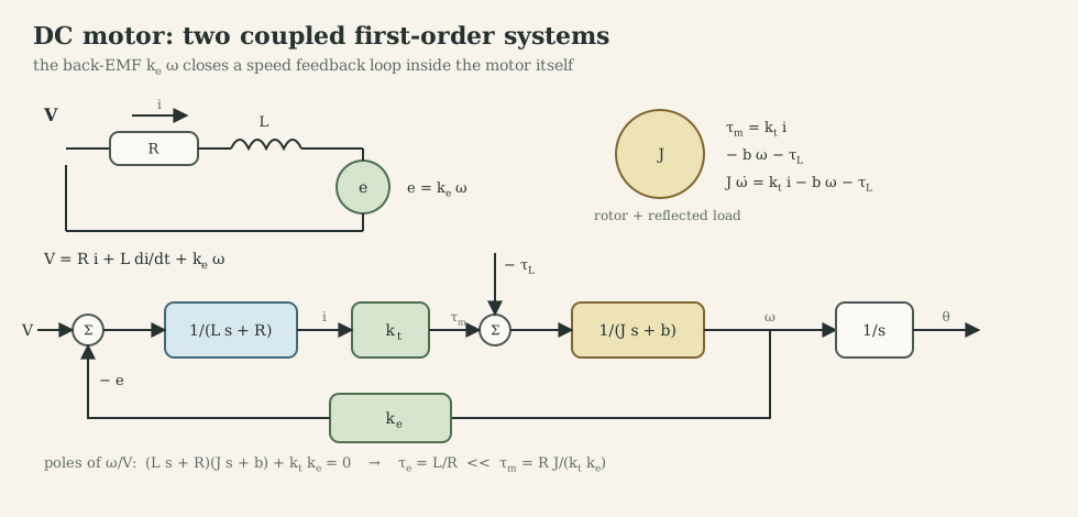
The block diagram shows the essential feature: the back-EMF closes a speed feedback loop inside the motor. At constant voltage, if the load slows the rotor, the back-EMF drops, the current rises and the torque recovers. This “electrical damping” $k_tk_e/R$ is usually much larger than mechanical friction $b$ in small motors (BX4: $k_tk_e/R=1.3\cdot10^{-3}$ N·m·s/rad versus $b\approx1.2\cdot10^{-5}$).
State space. With $x=[i,\ \omega]^\top$, input $u=V$, disturbance $w=\tau_L$:
\[\dot x=\underbrace{\begin{bmatrix}-R/L & -k_e/L\\ k_t/J & -b/J\end{bmatrix}}_{A}x+\underbrace{\begin{bmatrix}1/L\\0\end{bmatrix}}_{B}V+\underbrace{\begin{bmatrix}0\\-1/J\end{bmatrix}}_{E}\tau_L,\qquad y=Cx .\]With position, $x=[\theta,\ \omega,\ i]^\top$ adds a pure integrator. The choice of $C$ is the choice of sensor: $C=[0\ 1]$ for a tachometer or encoder-derived speed, $C=[1\ 0]$ for a current sensor, $C=[1\ 0\ 0]$ for an encoder in the 3-state model.
D.5 Transfer functions
Taking Laplace transforms with zero initial conditions:
\[\frac{\Omega(s)}{V(s)}=\frac{k_t}{(Ls+R)(Js+b)+k_tk_e},\qquad \frac{I(s)}{V(s)}=\frac{Js+b}{(Ls+R)(Js+b)+k_tk_e},\] \[\frac{\Omega(s)}{T_L(s)}=-\frac{Ls+R}{(Ls+R)(Js+b)+k_tk_e},\qquad \frac{\Theta(s)}{V(s)}=\frac{1}{s}\frac{\Omega(s)}{V(s)} .\]All share the characteristic polynomial $LJs^2+(RJ+bL)s+(Rb+k_tk_e)$. Three facts follow:
- Static speed gain $\omega/V=k_t/(Rb+k_tk_e)\approx1/k_e$: at no load the motor runs at the speed where back-EMF balances the supply.
- Static stiffness $\partial\omega/\partial\tau_L=-R/(Rb+k_tk_e)\approx-R/(k_tk_e)$: the slope of the torque-speed line. For the BX4 this is 766 rad/s per N·m = 7.3 rpm/mN·m, exactly the datasheet’s “slope of n-M curve”; for the Assun motor, 251 rpm/mN·m against the datasheet’s 252.3. The model and the datasheet agree.
- Current transfer has a zero at $-b/J$: a voltage step produces an inrush current that decays as the rotor accelerates (the back-EMF builds up).
D.6 Poles, time constants and the reduced model
The two poles separate widely when $\tau_e=L/R$ is much smaller than $\tau_m=RJ/(k_tk_e)$:
\[s_1\approx-\frac{R}{L},\qquad s_2\approx-\frac{k_tk_e}{RJ}\quad(\tau_e\ll\tau_m).\]| Motor (source) | $R$ | $L$ | $k_t=k_e$ | $J$ | $\tau_e=L/R$ | $\tau_m$ | Exact poles |
|---|---|---|---|---|---|---|---|
| Faulhaber 3268 BX4, 24 V (MF2030 datasheet) | 1.45 Ω | 110 µH | 0.0435 | 6.0·10⁻⁶ | 76 µs | 4.6 ms | −12 961 and −221 s⁻¹ |
| Assun AM-CL1643MB-1210, 12 V (MF2103 datasheet) | 3.42 Ω | 0.21 mH | 0.0114 | 3.11·10⁻⁷ | 61 µs | 8.2 ms | – |
| MF2007 workshop motor (identified) | 112 Ω | 11.4 mH | 0.0697 | 2.6·10⁻⁵ | 0.10 ms | 0.40 s* | – |
* including the identified viscous friction $d_m=2.15\cdot10^{-5}$ N·m·s/rad, which is significant for this motor.
When the separation is a factor of 50 or more, setting $L=0$ gives the reduced first-order model
\[\frac{\Omega(s)}{V(s)}=\frac{k_t/(RJ)}{s+(k_tk_e+Rb)/(RJ)},\]which the MF2030 report used after its pole analysis and the MF2007 workshop used for identification ($23.94/(s+2.495)$ for the workshop motor). When does the reduction fail? When the current is controlled (the current loop acts on exactly the dynamics that were dropped), when the PWM period is comparable to $\tau_e$ (Part J.7), and when designing anything above roughly $1/(10\tau_e)$ in bandwidth.
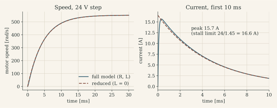
The simulation reproduces the MF2030 verification table: peak current 15.7 A (theoretical stall 16.6 A), no-load speed 551 rad/s (datasheet 576 rad/s, which includes the 0.215 A no-load current), initial acceleration 113.7·10³ rad/s² (datasheet 120·10³) and mechanical time constant 4.6 ms. Such a check is cheap and catches unit errors before any controller is designed.
D.7 Equilibria, controllability and observability
Equilibria. For constant $V$ and $\tau_L$: $\omega^\ast=(k_tV-R\tau_L)/(Rb+k_tk_e)$, $i^\ast=(b\omega^\ast+\tau_L)/k_t$. The model is linear, so there is one equilibrium per input; with Coulomb friction a dead band appears around $\omega=0$ (small voltages do not move the rotor at all, which the MF2007 identification observed at low amplitude).
Controllability. \(\mathcal C=[B\ AB]=\begin{bmatrix}1/L&-R/L^2\\0&k_t/(JL)\end{bmatrix}\) has determinant $k_t/(JL^2)\neq0$: the voltage can place both poles anywhere. Physically, the voltage reaches speed through current.
Observability depends on the sensor:
| Measured | Observability matrix | Conclusion |
|---|---|---|
| speed $\omega$ | \(\begin{bmatrix}0&1\\k_t/J&-b/J\end{bmatrix}\), det $=-k_t/J$ | current can be estimated from speed |
| current $i$ | \(\begin{bmatrix}1&0\\-R/L&-k_e/L\end{bmatrix}\), det $=-k_e/L$ | speed can be estimated from current and voltage: the basis of sensorless control |
| position $\theta$ (3 states) | full rank | everything is observable from an encoder |
| speed only (3 states) | rank 2 | absolute position is not observable from speed |
The second row is the theory behind sensorless control: back-EMF is observable through $V-Ri-L\,di/dt$, as long as the speed is high enough for $k_e\omega$ to stand out above the modelling errors in $R$ and the voltage.
D.8 Measured motor: identification in MF2007
The MF2007 workshops ran Simulink in external mode on a TI LAUNCHXL-F28379D (dual-core C2000, 200 MHz), driving a DC motor with a 3600 ppr encoder through a ±24 V power stage.
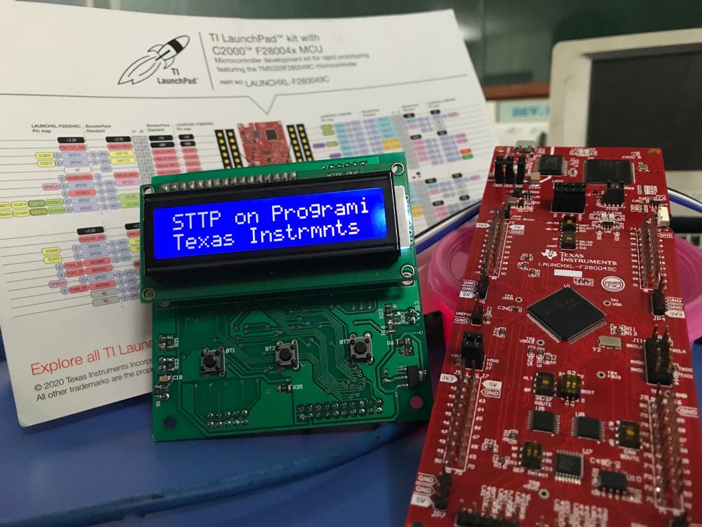
Method. Electrical parameters ($R$, $L$, $k_m$) from the datasheet; mechanical parameters ($J$, $d_m$, $F_c$) from experiments.
- Apply voltage steps of 7, 12 and 18 V. For the reduced model, the steady-state speed gives $k_m/(d_mR+k_ek_m)$ and the 63 % time gives $\tau=JR/(d_mR+k_ek_m)$.
- Fit $J$ and $d_m$ until the model speed matches the encoder speed for all three steps; validate with a 0.5 rad/s sine input. Result (level 1): $d_m=2.15\cdot10^{-5}$ N·m·s/rad, $J=2.6\cdot10^{-5}$ kg·m².
- The linear model fitted large inputs but left steady-state errors at low voltage. Adding Coulomb friction $M_f=d_m\omega+F_c\,\mathrm{sign}(\omega)$ fixed this with $F_c=1.35\cdot10^{-3}$ N·m (level 2).
The same identification as a least-squares problem. Sampling the reduced model with zero-order hold at $T_s$ gives
\[\omega_{k+1}=a\,\omega_k+\beta\,V_k-\gamma\,\mathrm{sign}(\omega_k),\]which is linear in the unknowns $(a,\beta,\gamma)$. Stacking $N$ samples gives $\mathbf y=\Phi\boldsymbol\vartheta$ and $\hat{\boldsymbol\vartheta}=(\Phi^\top\Phi)^{-1}\Phi^\top\mathbf y$ (solve it with QR, as discussed in the numerical linear algebra note). Then $a=e^{-T_s/\tau}$ gives $\tau$, and $\beta$, $\gamma$ give the gain and friction. Good practice: excite with several amplitudes (to separate Coulomb from viscous friction) and both directions, differentiate encoder position only after low-pass filtering, and validate on data not used for fitting.
D.9 Extending the model: the nutrunner drive train
The MF2030 project extended the motor model with the gearbox, shafts and nut into a 4th-order two-mass model (motor side angle $\theta_1$, nut angle $\theta_2$):
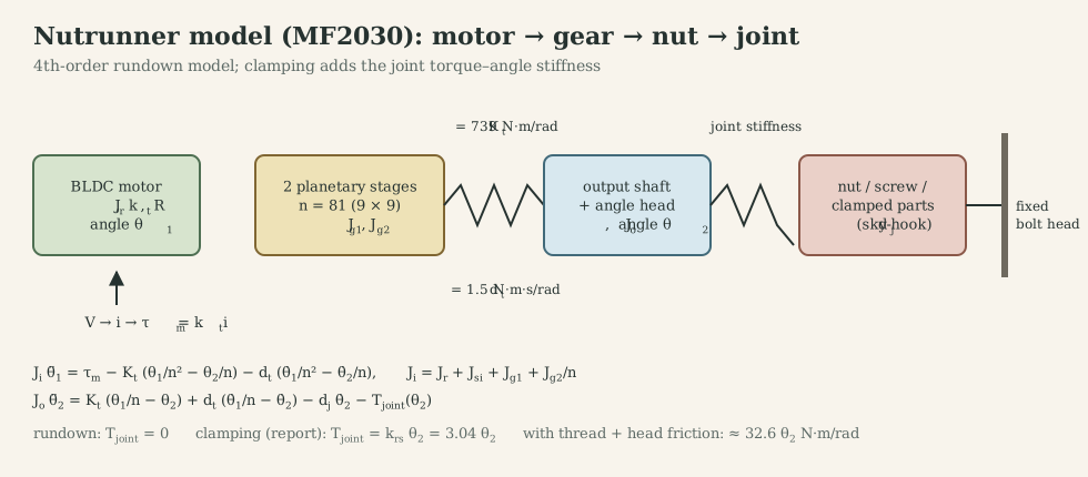
(The electrical pole is dropped, consistent with D.6.) With $x=[\theta_1,\theta_2,\dot\theta_1,\dot\theta_2]^\top$ this is a linear state-space model. Re-simulating it with the report’s parameters reproduces the report: a 1 V step gives 19.56 rad/s at the motor and 0.2415 rad/s at the nut, a ratio of exactly 81, with a 63 % rise time of about 4 ms.
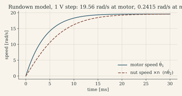
Two lessons from re-running it:
- The gearbox mode is extremely stiff. The eigenvalues are $-5.3\cdot10^5$ (gear coupling, overdamped by $d_t$) and $-238\pm67j$: in this parameter set the drive train behaves as one rigid body. A real nutrunner’s angle head and torque transducer are more compliant, and that compliance is what makes torque control interesting.
- Code and equations must agree. The MATLAB file for the clamping model uses the gearbox stiffness
Kt(739) in the input matrix where the torque constantkt(0.0435) belongs, a factor of about 17 000 in actuator gain, and the axial bolt stiffnesskj($7.7\cdot10^{7}$ N/m) where the rotational stiffnesskrs(3.04 N·m/rad) belongs. Both errors are invisible in the equations of the report and obvious in a unit check. The project page discusses their effect.
What to remember
- Two states (current, speed), one gyrator; the back-EMF is an inherent speed feedback.
- $\omega/V\approx1/k_e$ at no load; $\partial\omega/\partial\tau_L\approx-R/(k_tk_e)$ is the datasheet slope.
- $\tau_e\ll\tau_m$ justifies the first-order model for speed, never for current control.
- Speed measurement makes current observable and vice versa: the root of sensorless control.
- Identify $J$, viscous and Coulomb friction with multi-amplitude steps; solve by least squares; validate on fresh data.
Part E. Sensors: what the loop actually sees
A controller acts on measurements, not on the motor. Every sensor puts its own range, resolution, noise, bias and lag between the physical variable and the number the controller uses, and all of them sit inside the loop. This part defines the properties that matter, goes through the sensors a motor drive uses (encoders, Hall sensors, resolvers, current, voltage and torque sensors), and ends with the first estimation problem every drive meets: speed from a position sensor.
E.1 What makes a sensor good enough
| Property | Meaning | Example in my hardware |
|---|---|---|
| Range | span that can be measured without saturating | my lab-4 current sensor as drawn saturates near ±0.55 A |
| Resolution | smallest change that changes the output | 2048 counts/rev: 0.18° (MF2103); 12-bit ADC on 3.3 V: 0.81 mV |
| Accuracy | closeness to the true value: offset, gain error, nonlinearity | a 1 % shunt gives at least a 1 % torque error |
| Noise (precision) | spread of repeated readings | INA126: 35 nV/√Hz input noise at 1 kHz |
| Bandwidth | frequency up to which the output follows the input | INA126: 200 kHz at gain 5, 9 kHz at gain 100 |
| Latency | time from the physical event to the number in memory | ADC conversion of microseconds; speed by differencing: $T_s/2$ |
| Robustness | behaviour under temperature, EMI, vibration, dirt | optical encoders dislike dirt; resolvers tolerate it |
Two consequences hold for every sensor in a loop:
- The loop controls the sensor output, not the physical variable. A gain error in the sensor becomes a gain error in the controlled quantity; a bias becomes a steady-state error that no integrator can see. Calibration is part of control design.
- Sensor dynamics and noise are part of the loop. With a sensor model $G_s(s)$ the loop gain is $C\,G\,G_s$: the sensor’s lag reduces phase margin like any other delay, and its noise reaches the output through the complementary sensitivity $T$ (Part G.8). That is why sensor bandwidth should exceed loop bandwidth by about 5-10×, and why noise must be removed where the loop does not need gain.
Resolution, accuracy and bandwidth are independent. A 14-bit magnetic angle sensor can be resolution-rich and still carry a once-per-revolution error of 1° from magnet misalignment; a precise sensor can be useless in a current loop if it is too slow.
E.2 Incremental encoders and quadrature decoding
Principle. An optical encoder shines light through a slotted disc onto photodiodes; a magnetic encoder reads a magnetized ring or a diametric magnet with Hall or magnetoresistive elements. Either way, the output is two square waves A and B, each with $N$ periods (“lines”) per revolution, shifted by a quarter period (90° electrical), and often an index pulse Z once per revolution.
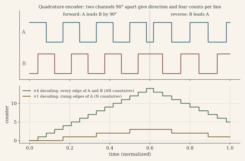
Quadrature decoding. The pair (A, B) steps through a Gray-code cycle 00 → 10 → 11 → 01 → 00 when turning forward and the reverse sequence when turning backwards. Each legal transition changes exactly one bit and moves the count by ±1; a transition where both bits change is illegal and means a missed edge (noise, or edges faster than the decoder can sample).
| Decoding | Counts on | Counts per rev | Use |
|---|---|---|---|
| ×1 | rising edge of A, direction from B | $N$ | simple counters |
| ×2 | both edges of A | $2N$ | rarely |
| ×4 | every edge of A and B | $4N$ | standard in timer encoder modes |
In the microcontroller. Counting is done in hardware, not in interrupts. The STM32’s general-purpose and advanced timers have an encoder interface mode with a digital input filter. In MF2103, TIM1 counted A/B on PA8/PA9 into a 16-bit counter that the speed loop simply read. The TI C2000 used in MF2007 has a dedicated eQEP peripheral that also latches the index and measures edge periods. A 16-bit counter wraps after 65 536 counts. Taking the difference of two readings in a 16-bit signed type handles the wrap automatically, as long as fewer than 32 768 counts pass between readings.
Limits and errors.
- Count rate: $f_{\text{edge}}=N_{\text{cpr}}\cdot\text{rpm}/60$. At 2048 counts/rev and 10 000 rpm that is 341 kHz; the timer input filter must pass it while rejecting glitches.
- Disc errors: eccentricity gives a once-per-revolution angle error; unequal A/B duty or a phase error other than 90° makes the four edges per line unevenly spaced. Speed computed from such counts carries a ripple at $4N$ times the rotation frequency.
- Electrical noise: a spike on a single-ended line is counted as an edge, and the position error accumulates. Differential (RS-422) line drivers, Schmitt-trigger inputs, short shielded cables and the decoder’s filter keep counts honest.
- No absolute reference: an incremental encoder knows only displacement since power-up. Homing to the index pulse, or an absolute encoder (multi-track Gray code, or a serial protocol such as SSI, BiSS or EnDat), gives absolute position.
Sin/cos encoders and interpolation. Some encoders output analog sine and cosine instead of square waves. An ADC samples both, and $\theta=\text{atan2}(\sin,\cos)$ locates the angle within a line. Interpolation by 100-1000× is common, limited by signal amplitude matching, offsets and ADC noise.
Case-study hook. The MF2007 parameter file sets plsPerRev = 3600 for the C2000 rig. The MF2103 firmware divides by 2048 counts/rev, a number not documented anywhere in the course material. A wrong counts-per-revolution constant is a pure gain error on speed, so the speed loop would regulate to the wrong speed without any visible error. The project page lists both as items to verify.
E.3 Hall sensors, resolvers and potentiometers
Hall-effect sensors. A current through a thin semiconductor plate in a magnetic field produces a transverse voltage $V_H=IB/(nqt)$. Digital Hall switches mounted in a brushless motor detect the rotor magnet: three sensors 120° (electrical) apart divide each electrical revolution into six sectors. That is exactly what six-step commutation needs (Part I.2), but the angle resolution is 60° electrical. For the BX4 with two pole pairs that means 12 sectors per mechanical revolution (30°), too coarse for smooth FOC or precise positioning without interpolation. Speed can be estimated from the time between Hall edges. Analog (linear) Hall sensors and 2D magnetic angle ICs with a diametric magnet give 12-14-bit absolute angle on one chip.
Resolvers. A resolver is a rotary transformer. An excitation winding fed at, say, 10 kHz induces two output voltages whose amplitudes are modulated by $\sin\theta$ and $\cos\theta$. A resolver-to-digital converter demodulates them and runs a tracking loop (a PLL, Part H.5) that outputs angle and speed. Resolvers have no electronics in the motor, tolerate heat, vibration and dirt, and give absolute angle within one revolution. That is why traction motors use them.
Potentiometers and tachogenerators. A potentiometer gives absolute angle as a voltage. It is cheap, but it wears, has a limited angle and needs an ADC with anti-alias filtering. MF2007’s implementation lecture uses one for the position of a cart. A tachogenerator is a small DC generator whose voltage is proportional to speed: it is analog, continuous and has commutator ripple. It is mostly historical, but it explains why “speed sensor” once meant a voltage.
| Sensor | Measures | Absolute? | Typical resolution | Strengths | Weaknesses |
|---|---|---|---|---|---|
| Incremental encoder | angle change | no (index once per rev) | $4N$ counts/rev, 500-40 000 | simple digital interface, hardware counting | needs homing; noise counts accumulate |
| Absolute encoder | angle | yes | 12-23 bit | position at power-up | cost, serial protocol latency |
| Sin/cos encoder | angle | within a line | interpolated, > 20 bit | very fine resolution | analog signal quality, ADC load |
| Hall switches (×3) | rotor sector | within electrical rev | 60° electrical | robust, cheap, built into BLDC | coarse |
| Magnetic angle IC | angle | within one rev | 12-14 bit | single chip, contactless | magnet alignment errors |
| Resolver | angle | within one rev | 12-16 bit after RDC | rugged, high temperature | excitation and demodulation electronics |
| Potentiometer | angle | yes | analog (ADC-limited) | trivial | wear, limited angle, noise |
| Tachogenerator | speed | – | analog | continuous speed | ripple, size, drift |
E.4 Current, voltage and torque sensors
Current. Torque follows current ($\tau=k_ti$), so the current sensor is the torque sensor of an electric drive. Two families:
- Shunt + amplifier. A small resistor $R_S$ gives $v=R_Si$. An instrumentation or current-sense amplifier with gain $G$ and an offset $V_{\text{ref}}$ maps it onto the ADC: $v_{\text{ADC}}=V_{\text{ref}}+G R_S\,i$. Design backwards from the ADC: for a 0-3.3 V input and a bidirectional range $\pm i_{\max}$, choose $V_{\text{ref}}=1.65$ V and $GR_S=1.65\ \text{V}/i_{\max}$ (1.1 V/A for ±1.5 A). Taking $V_{\text{ref}}$ from the same reference as the ADC makes the measurement ratiometric, so reference drift cancels. The shunt dissipates $i^2R_S$ (0.23 W for 0.1 Ω at 1.5 A) and should be read with a Kelvin (four-wire) connection.
- Hall-effect current sensors. A magnetic core concentrates the conductor’s field onto a Hall element. Open-loop types are simple; closed-loop (compensated) types null the core flux with a secondary winding for better linearity. Both are galvanically isolated and lossless, at the cost of offset drift, limited bandwidth and price.
Where the shunt sits relative to the bridge (low side, high side, in the phase) decides what it can see and what common-mode voltage the amplifier must reject. That belongs to the power stage and is treated in Part J.8. The amplifier’s dynamics matter too. An instrumentation amplifier’s bandwidth falls with gain: the INA126 has 200 kHz at $G=5$ and 9 kHz at $G=100$, about 1 MHz gain-bandwidth. Its slew rate (0.4 V/µs) limits how fast the output can follow PWM edges.
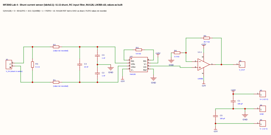
Case-study hook. My MF2043 lab-4 sensor (0.1 Ω, INA126 at $G=19.3$, LM358 stage ×10) gives 19.3 V/A with the reference pin grounded. A 3.3 V ADC therefore sees only 0-0.17 A, and negative currents are lost. Designing backwards from the ADC would have given about 1.1 V/A around 1.65 V. The project page has the full netlist review.
Voltage. A resistive divider, filtered, measures the DC bus. The controller needs it: dividing the voltage command by the measured bus voltage, $D=v^\ast/V_{\text{bus}}$, keeps the loop gain constant while a battery discharges.
Torque. A torque transducer is a shaft with strain gauges in a Wheatstone bridge, with an output of a few mV/V. It needs a precision amplifier and, on a rotating shaft, slip rings or telemetry. In a tightening tool it measures the controlled variable directly. The alternative is to estimate output torque from motor current, $\eta n k_t i$. That is cheap, but gearbox efficiency varies by 10-20 % with load, speed and temperature, so tools that must prove the torque they delivered carry a transducer. In other words, a sensor is used where the model is not trusted.
Temperature. An NTC thermistor in the winding or on the power stage feeds a thermal model ($I^2t$ protection, Part J.10). Because winding resistance rises about 0.39 %/K, the measured temperature also corrects $R$ in current-loop and sensorless models.
E.5 From position to speed
Most drives measure angle and need speed. Differentiating a quantized signal is the first estimation problem of the loop. There are three classical answers, each a different compromise:
M-method (count edges in a fixed window).
\[\hat\omega_k=\frac{2\pi}{N_{\text{cpr}}}\,\frac{n_k-n_{k-1}}{T_s},\qquad \Delta\omega=\frac{2\pi}{N_{\text{cpr}}T_s}.\]The quantum $\Delta\omega$ is fixed, so the relative error shrinks with speed: good at high speed, poor at low speed. With MF2103’s 2048 counts/rev, one count per period is 0.59 rpm at 50 ms, 2.93 rpm at 10 ms and 29.3 rpm at 1 kHz. With MF2007’s 3600 counts at 2 ms it is 0.87 rad/s. Faster loops see a coarser speed. The estimate is the average speed over the last period, so it lags by $T_s/2$ and behaves like a moving-average filter.
T-method (time the edges). Capture the time between two consecutive edges with a fast timer clock $f_{\text{clk}}$:
\[\hat\omega=\frac{2\pi}{N_{\text{cpr}}}\,\frac{f_{\text{clk}}}{m},\]where $m$ is the number of timer ticks between edges. The relative error is about $1/m$, so it is excellent at low speed (many ticks per edge) and poor at high speed. It has two weaknesses: at standstill no edge arrives, so the estimate must time out; and it reports the speed of the last edge, not the present one.
M/T method. Count the edges in the window and time the first and last edge exactly: $\hat\omega=2\pi\,\Delta n/(N_{\text{cpr}}\,\Delta t_{\text{edges}})$. This is accurate over the whole range and is what C2000 eQEP and similar capture units support.
Where M and T are equally good. Equating the relative resolutions $1/\Delta n$ and $1/m$ gives
\[\omega^\ast=\frac{2\pi}{N_{\text{cpr}}}\sqrt{\frac{f_{\text{clk}}}{T_s}} .\]For 2048 counts/rev, a 1 MHz capture clock and $T_s=1$ ms, that is 97 rad/s (930 rpm): below it, time the edges; above it, count them.
Filtering and model-based estimation. Low-pass filtering the M-method estimate removes quantization noise but adds lag. A first-order filter at $f_c$ delays slow signals by about $1/(2\pi f_c)$, 8 ms at 20 Hz, so a ramp is reported late. The better answer uses information the controller already has: it knows the torque it commands. An observer or Kalman filter (Part H) predicts the speed from the current and corrects the prediction with the counts. It then sees through quantization without the lag of a filter, and estimates the load torque as a by-product. Figure H.3 compares all four methods on the same data.
What to remember
- The loop controls the sensor’s output: sensor gain errors and biases become control errors; sensor lag and noise sit inside the loop.
- Quadrature encoders give direction and $4N$ counts per revolution; count in hardware; handle counter wrap with a signed difference; protect the lines against noise.
- Hall sensors give six sectors per electrical revolution (enough to commutate, not to servo); resolvers and absolute encoders give absolute angle.
- Design current sensors backwards from the ADC range, bidirectional around a ratiometric mid-scale reference.
- Speed from counts: count edges at high speed, time edges at low speed, or combine both; a model-based estimator removes quantization without filter lag.
Part F. The signal chain: sampling, filters, ADC, DAC and PWM
Between the sensor and the controller, and again between the controller and the power stage, the signal crosses the boundary between the continuous and the discrete world. Four things happen there, and each has its own rule: sampling (what is lost and what is invented, F.1), filtering before the sampler (which cut-off frequency, F.2), analog-to-digital conversion (resolution, sample-and-hold, triggering, F.3) and digital-to-analog conversion, where in a drive the DAC is usually a PWM timer (F.4). Part G then uses these results to choose the sampling rate of every loop.
F.1 Sampling, aliasing and the Nyquist frequency
What sampling does. Sampling $x(t)$ every $T_s$ keeps only $x(kT_s)$. In the frequency domain, the spectrum of the sampled signal is the original spectrum repeated at every multiple of $f_s=1/T_s$:
\[X_s(f)=\frac{1}{T_s}\sum_{k=-\infty}^{\infty}X(f-kf_s).\]Two facts follow.
- Nyquist-Shannon. If $x$ contains nothing at or above the Nyquist frequency $f_N=f_s/2$, the copies do not overlap and the samples determine $x$ completely.
- Aliasing. A component at $f>f_N$ lands, after sampling, at
where it is indistinguishable from a genuine signal at that frequency. No digital processing can undo it, because the information about which frequency it came from is gone. MF2007’s example: a 0.9 Hz sine sampled at 1 Hz gives exactly the samples of $-\sin(2\pi\cdot0.1\,n)$, a 0.1 Hz signal.
Aliases in a motor drive.
| Signal | True frequency | Sampled at | Appears at | Consequence |
|---|---|---|---|---|
| PWM current ripple | 20 kHz | free-running ADC at 9.9 kHz | 200 Hz | a fake 200 Hz oscillation in the measured current; the current loop “corrects” it and injects real 200 Hz torque ripple |
| PWM current ripple | 20 kHz | 10 kHz, synchronized to the PWM | 0 Hz (DC) | a constant bias whose size depends on the sampling instant |
| Six-step torque ripple of the BX4 at 243 rad/s | 6 × 77 Hz = 464 Hz | 100 Hz outer loop | 36 Hz | a slow “oscillation” in the angle loop that does not exist |
| Mains interference on a sensor cable | 50 Hz | 1 kHz speed loop | 50 Hz | no alias, but noise inside the speed-loop bandwidth: shield the cable or filter |
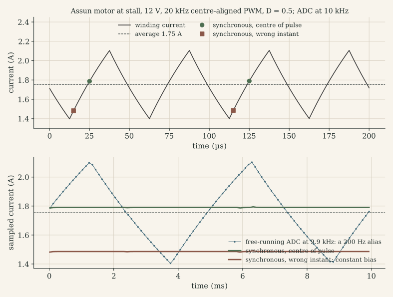
Synchronous sampling is aliasing on purpose. Sampling once per PWM period (or every second period) at a fixed phase folds every PWM harmonic onto DC. Choosing the phase where the ripple crosses its average makes that DC value the average current. In centre-aligned PWM that instant is the middle of the on- or off-interval. This is why drives trigger the ADC from the PWM timer (Part M.5) instead of filtering the ripple away.
Case-study hook: three sampling frequencies in one lab. My MF2043 lab-3 material (the filter prestudy, the course’s mbed sampling program and the MATLAB real-time plotter) shows how easily $f_s$ gets lost:
- the prestudy asks for filters designed for $f_s=8$ kHz;
- the mbed program samples with a 50 µs
Ticker, i.e. 20 kHz, and sends one byte per sample at 921 600 baud; - the plotter sets
data.f = 80000.
If the program and the plotter are used as they are, every time axis is compressed four times and every FFT frequency reads four times too high: a 1 kHz test tone appears at 4 kHz. The program comment says “Match data.f in Matlab”, which shows how easy the mismatch is to make. The serial link sets a hard ceiling: 921 600 baud at 10 bits per byte carries at most 92 160 samples/s, so 80 kHz would use 87 % of it. The program also scales the 0-1 reading to 8 bits (12.9 mV steps on 3.3 V) to fit one byte. Define $f_s$ once, in one place, and store it with the data.
F.2 Cut-off frequency and anti-aliasing filters
Cut-off frequency. A first-order low-pass $H(s)=1/(1+s/\omega_c)$ with $\omega_c=2\pi f_c=1/(RC)$ passes low frequencies and attenuates high ones. At $f_c$:
- $\lvert H\rvert=1/\sqrt2$, i.e. −3 dB (half the power);
- the phase is −45°.
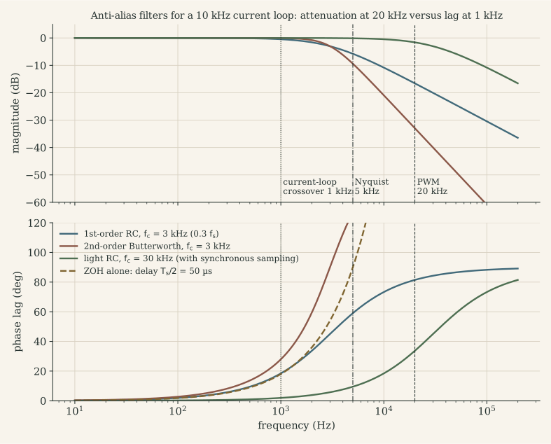
Below $f_c$ the filter costs phase, $\varphi(f)=-\arctan(f/f_c)$, which for $f\ll f_c$ is a pure delay of $1/\omega_c$. Above $f_c$ it attenuates by 20 dB per decade. Higher-order filters roll off faster (20n dB/decade for order n) and lag more in the passband:
| Filter | Attenuation per decade above $f_c$ | Phase lag at $f_c/10$ | Phase lag at $f_c/3$ | Low-frequency delay |
|---|---|---|---|---|
| 1st order RC | 20 dB | 5.7° | 18.4° | $1/\omega_c$ |
| 2nd order Butterworth ($Q=0.707$) | 40 dB | 8.1° | 27.9° | $\sqrt2/\omega_c$ |
| Moving average over $M$ samples (digital) | nulls at multiples of $f_s/M$ | – | – | $(M-1)T_s/2$ |
The cut-off frequency is therefore a trade-off between what the filter removes above $f_c$ and what it costs the loop below $f_c$.
Why an analog filter, before the ADC. Only a filter before the sampler can prevent aliasing. After sampling, the alias is already inside the band. MF2007’s rule: never close a feedback loop through an ADC without an anti-aliasing filter on every analog input. Digital sensors such as encoders do not alias in the same way, because counting edges is not point sampling.
Choosing the cut-off: the MF2007 recipe.
- Make a preliminary continuous design and find the fastest frequency $\omega_b$ among the plant, the controller and the closed loop.
- Choose $\omega_s\in[10,30]\,\omega_b$ (Part G.10).
- Choose the anti-alias bandwidth $\omega_a\in[0.2,0.33]\,\omega_s$.
- If $\omega_a$ is close to the closed-loop poles, include the filter in the plant model and redesign.
My group’s MF2007 parameter file does exactly this: wa = 0.3*ws and Ga = 1/(s/wa+1), discretized with Tustin. At $T_s=2$ ms that is $\omega_a=942$ rad/s (150 Hz), costing 1.5° at the 24 rad/s speed-loop bandwidth. Because the rig measured position with an encoder, this filter smoothed quantization noise rather than preventing aliasing.
How much attenuation is enough? To push an out-of-band component of amplitude $A$ below one LSB of the ADC, the filter needs $\lvert H(f)\rvert\le\text{LSB}/A$. For the 0.71 A peak-to-peak ripple of the MF2103 motor at 20 kHz, on a ±1.5 A, 12-bit current channel (0.73 mA per LSB), that is 0.73 mA / 0.36 A, i.e. −54 dB at 20 kHz. A first-order filter reaches that only with $f_c\approx41$ Hz, a second-order one with $f_c\approx0.9$ kHz. Both are useless for a current loop with 1 kHz bandwidth. That is the quantitative reason drives remove ripple by synchronous sampling (F.1) and keep only a light RC filter, with a cut-off far above the loop bandwidth, against switching spikes.
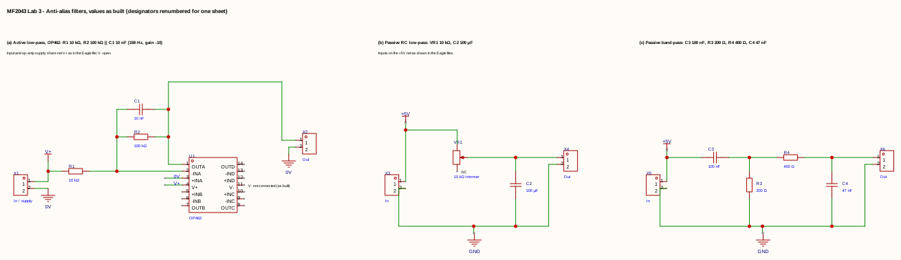
The filters on my boards, as drawn. All values are from the Eagle schematics; the project page has the netlists.
| Board | Topology | Values | Cut-off | Comment |
|---|---|---|---|---|
| Lab 3, passive low-pass | trimmer in series, capacitor to ground | 0-10 kΩ trimmer, 100 µF | ≥ 0.16 Hz | with 100 µF the cut-off is below 0.2 Hz at any trimmer setting; for $f_s=8$ kHz and $f_c\approx0.3f_s$ with 10 kΩ, about 6.8 nF is needed |
| Lab 3, active low-pass | inverting OP462 stage, $R_2\parallel C$ in feedback | 10 kΩ in, 100 kΩ ∥ 10 nF | 159 Hz, gain −10 | inverting with gain 10, so a 0-3.3 V input drives the output negative; an ADC input needs unity gain and a mid-supply reference, or a non-inverting Sallen-Key stage |
| Lab 3, passive band-pass | series C, shunt R, series R, shunt C | 100 nF, 200 Ω, 400 Ω, 47 nF | corners 8.0 and 8.5 kHz | the stages load each other: peak −7.6 dB at 8.2 kHz, −3 dB band 2.9-23 kHz |
| Lab 4, current-sensor input | series R per input, 1 nF to ground each, 10 nF across | R not recorded | differential $1/(2\pi\cdot2R(C_d+C_c/2))$: 76 kHz for R = 100 Ω (assumed) | RF and spike filter; $C_d\ge10\,C_c$ so capacitor mismatch does not convert common-mode noise into a differential error |
Digital filters after the ADC. Once the signal is clean of aliases, a digital low-pass can trade noise for lag inside the band. The first-order IIR
\[y_k=y_{k-1}+\alpha\,(x_k-y_{k-1}),\qquad \alpha=1-e^{-\omega_cT_s}\]costs one multiply-add (MF2043 lab 3 asks for one with $f_c=200$ Hz). A moving average over one PWM period places a notch at the PWM frequency and its harmonics. The phase lag of every filter must be counted in the loop.
F.3 The ADC: from volts to numbers
Successive approximation (SAR). Microcontroller ADCs are almost always SAR converters, and a conversion has two phases:
- Sampling (acquisition). A switch connects the input to a small internal capacitor $C_{\text{ADC}}$ (a few pF) for a programmable sampling time. The capacitor must charge to within ½ LSB of the input. The instant the switch opens is the sampling instant: this is what a timer trigger sets.
- Conversion. With the switch open (hold), a binary search compares the held charge against an internal capacitive DAC, one bit per clock: 12 bits take about 12.5 ADC clocks. The input may change during conversion; only the sampling window matters.
Settling and source impedance. Charging $C_{\text{ADC}}$ through the source resistance $R_{\text{src}}$ (plus the switch resistance) to ½ LSB of an N-bit converter takes
\[t_{\text{sample}}\ \ge\ (R_{\text{src}}+R_{\text{sw}})\,C_{\text{ADC}}\,\ln\!\left(2^{N+1}\right).\]For 12 bits, $\ln 2^{13}=9.0$. With an assumed $C_{\text{ADC}}=5$ pF and a 10 kΩ divider, that is 0.45 µs, or 36 clocks at 80 MHz: a high-impedance source needs a long sampling time. An op-amp output (like the LM358 stage of my lab-4 sensor) or a capacitor at the pin removes the problem. For charge sharing to stay below ½ LSB, the capacitor needs $C_{\text{ext}}\ge2^{N+1}C_{\text{ADC}}$, about 40 nF. Its RC with the source resistance then becomes the anti-alias filter. Look up the actual $C_{\text{ADC}}$ and the table of maximum source impedance in the datasheet.
Resolution and quantization noise. With reference $V_{\text{ref}}$ and $N$ bits,
\[\text{LSB}=\frac{V_{\text{ref}}}{2^N},\qquad e_{\text{rms}}=\frac{\text{LSB}}{\sqrt{12}},\qquad \text{SNR}_{\text{ideal}}=6.02N+1.76\ \text{dB}.\]For 12 bits on 3.3 V: 0.81 mV per LSB, 0.23 mV rms, 74 dB. Real converters lose 1-2 bits to noise, offset and nonlinearity, expressed as the effective number of bits $\text{ENOB}=(\text{SINAD}-1.76)/6.02$. Converted to physical units through the sensor gain:
| Channel | Scale | One LSB (12 bit) | In motor terms |
|---|---|---|---|
| Lab-4 sensor as drawn, 19.3 V/A from 0 V | 0-0.17 A on 0-3.3 V | 42 µA | too little range for any motor current |
| Same shunt redesigned, 1.1 V/A around 1.65 V | ±1.5 A | 0.73 mA | 0.03 mN·m for the BX4 ($k_t$ = 43.5 mN·m/A) |
| Nutrunner current channel (Part Q) | ±12 A | 5.9 mA | 0.26 mN·m at the motor |
| Bus voltage via 1:11 divider | 0-36 V | 8.9 mV | 0.04 % of a 24 V bus |
Offset and gain errors. An offset of a few LSB in a current channel is a constant torque error. In FOC it becomes a torque ripple at the electrical frequency, because the offset rotates with the Park transform. Measure offsets at standstill with the PWM off, and use the ADC’s self-calibration (STM32 ADCs have one).
Oversampling. Averaging $M$ samples reduces white noise by $\sqrt M$ and gains $\tfrac12\log_2M$ bits, but only if the noise is at least about 1 LSB (dither). Without noise, averaging identical codes gains nothing. The STM32L476’s ADC can do this in hardware (2× to 256×, with a programmable right shift), reaching 16 bits at 256×. The price is time ($M$ conversions) and a moving-average filter with its own delay.
Triggering and timing. In a drive the ADC is started by the PWM timer (a TRGO or compare event), not by software, so the sampling instant is fixed relative to the switching (F.1). STM32 injected channels convert a short group of channels on a hardware trigger and raise one interrupt at the end; the control ISR runs on that interrupt (Part N.7). Simultaneous sampling of two phase currents needs two ADCs triggered together; a single multiplexed ADC samples them some microseconds apart.
Case-study hook. The STM32L476 on the MF2103 board has three 12-bit SAR ADCs (5 Msps, hardware oversampling to 16 bits) and two 12-bit DAC channels. The MF2103 project used none of them; the loop was closed on the encoder alone. That is why a current loop is the first item of the project page’s next steps.
F.4 The output side: DAC, PWM and reconstruction
The zero-order hold. A DAC, or a PWM timer, holds each output value for one sampling period. As a filter the hold has the frequency response
\[H_{\text{ZOH}}(j\omega)=e^{-j\omega T_s/2}\,\frac{\sin(\omega T_s/2)}{\omega T_s/2}:\]a delay of half a period (phase lag $\omega T_s/2$, i.e. $180°\cdot f/f_s$) and a gentle amplitude droop (−3.9 dB at Nyquist). At a crossover a tenth of the sampling rate, the hold alone costs 18°. The images of the signal at multiples of $f_s$ must be removed by a reconstruction filter, which in a drive is the plant itself.
Real DACs. Resistor-string, R-2R ladder or capacitive converters output a voltage that settles within microseconds. In a drive they are mainly used for:
- Instrumentation. Writing an internal variable (current error, estimated angle) to a DAC pin lets an oscilloscope show it in real time next to the analog signals. It is the cheapest real-time debugging tool there is (Part O.3).
- Analog references. A DAC (or filtered PWM) on the REF pin of my lab-2 A4973 bridge sets its chopper current limit, $I_{\text{trip}}=V_{\text{REF}}/(2R_S)$. That turns the driver into a hardware current controller with a programmable setpoint, which is how stepper drivers microstep.
- Protection thresholds. A DAC feeding an internal comparator, whose output drives the timer’s break input, gives over-current shutdown in hardware within a microsecond, independent of software.
PWM as a DAC. A PWM output is a 1-bit DAC whose average is $D\,V_{\text{bus}}$. Its resolution is set by the timer:
\[N_{\text{bits}}=\log_2\frac{f_{\text{clk}}}{f_{\text{PWM}}}\ \ \text{(edge-aligned)},\qquad \log_2\frac{f_{\text{clk}}}{2f_{\text{PWM}}}\ \ \text{(centre-aligned)}.\]MF2103’s TIM3 at 40 MHz and 20 kHz has 2000 steps (11 bits): 0.05 % duty, 6 mV on a 12 V bridge. At 100 kHz the same clock gives 400 steps (8.6 bits), and on a 24 V bus one step is 60 mV. Across a 1.45 Ω winding that is a 41 mA current step, which can make a current loop limit-cycle between two duty values. Dithering the least significant bit, or sigma-delta modulation of the duty, recovers resolution at the cost of noise.
Who reconstructs the signal. The winding is the first reconstruction filter, a low-pass with corner $R/(2\pi L)$:
- 2.1 kHz for the BX4;
- 2.6 kHz for the MF2103 coreless motor;
- 1.6 kHz for the MF2007 motor.
PWM at 20 kHz is only 8-12 times above these corners, which is why the current ripple is large (Part J.7). The rotor inertia is the second filter; its mechanical corner is tens of hertz, so speed hardly sees the ripple. For an analog output (a reference voltage, a test signal), an RC after the PWM pin plays this role. With $\tau=RC$ the peak-to-peak ripple at 50 % duty is about $V T_{\text{PWM}}/(4\tau)$ and the settling time is about $5\tau$. A 20 kHz PWM on 3.3 V with $f_c=200$ Hz gives 52 mV ripple and 4 ms settling: faster settling costs more ripple.
Nonlinearity of the bridge. Dead time makes the PWM DAC nonlinear: during the dead time the current’s direction, not the gate signal, decides the output voltage. The resulting voltage error is
\[\Delta V\approx\operatorname{sign}(i)\,t_{\text{dead}}\,f_{\text{PWM}}\,V_{\text{bus}} .\]With the A4973’s 500 ns crossover dead time at 20 kHz on 24 V, that is 0.24 V, 1 % of the bus. It is invisible at high duty, dominant near zero current, and it distorts low-speed operation. The remedy is to add $\operatorname{sign}(\hat i)\,\Delta V$ to the voltage command.
What to remember
- Sampling copies the spectrum at multiples of $f_s$; anything above $f_s/2$ aliases and cannot be removed afterwards.
- Synchronous sampling at the right PWM phase is the drive’s anti-aliasing for current; free-running ADCs turn ripple into fake low-frequency signals.
- The cut-off frequency is a trade-off: attenuation above it versus phase lag below it. MF2007’s recipe is $\omega_s=(10\text{-}30)\,\omega_b$ and $\omega_a=(0.2\text{-}0.33)\,\omega_s$, with the filter included in the design if it comes close to the closed-loop poles.
- An ADC samples at the instant the hold switch opens; the source must settle $C_{\text{ADC}}$ within the sampling time; LSB, quantization noise and ENOB set the useful resolution in physical units.
- The output side is a zero-order hold with half a period of delay; PWM is a DAC with $\log_2(f_{\text{clk}}/f_{\text{PWM}})$ bits; the winding and the inertia are its reconstruction filters; dead time makes it nonlinear near zero current.
Part G. Feedback control: continuous and discrete
Every controller below is a different answer to the same question: which state do we feed back, and what does that feedback physically change in the motor? The DC motor model of Part D is the plant throughout; numbers come from the three motors.
G.1 Open-loop voltage drive
Applying a constant voltage already gives a stable speed (the back-EMF loop of D.4), with steady state $\omega\approx V/k_e$ and droop $-R/(k_tk_e)$ per unit load torque. Open loop is adequate for fans and toys. Its weaknesses: speed depends on load and supply voltage, the inrush current at start-up is $V/R$ (16.6 A for the BX4 at 24 V, ten times its continuous rating), and nothing limits torque.
G.2 Current (torque) control
Since $\tau_m=k_ti$, controlling current is controlling torque. From the voltage equation, the current sees the plant
\[\frac{I(s)}{V(s)-E(s)}=\frac{1}{Ls+R},\]with the back-EMF $E=k_e\omega$ acting as a slowly varying disturbance (the mechanical time constant is much longer than the electrical one).
PI with pole-zero cancellation. Choose $C_i(s)=K_p+K_i/s=K_p(s+K_i/K_p)/s$ with $K_i/K_p=R/L$, so the controller zero cancels the electrical pole. The open loop becomes $K_p/(Ls)$ and the closed loop
\[\frac{I}{I^\ast}=\frac{1}{1+s/\omega_c},\qquad K_p=\omega_cL,\quad K_i=\omega_cR .\]For the BX4 with a 1 kHz current-loop bandwidth ($\omega_c=6283$ rad/s): $K_p=0.69$ V/A, $K_i=9.1\cdot10^3$ V/(A·s).
Back-EMF feedforward. Adding $\hat e=k_e\hat\omega$ to the controller output removes the disturbance the integrator would otherwise chase; in FOC the same idea becomes cross-coupling decoupling (Part I.5).
What it physically changes. The current loop turns a voltage-driven motor (speed-like source) into a current-driven one (torque source). The back-EMF damping disappears from the outer loops’ point of view, inrush current is limited by the current reference clamp, and the plant for the speed loop becomes a pure inertia.
Limits. Bandwidth must stay well below the sampling rate (Part G.10) and the PWM frequency; the voltage saturates at $\pm V_{\text{bus}}$, so at high speed little voltage margin remains to change current quickly.
G.3 Velocity control
With a current loop inside, the speed loop sees
\[\frac{\Omega(s)}{I^\ast(s)}\approx\frac{k_t}{Js+b}\](current-loop dynamics neglected if 5-10 times faster). A PI controller places both closed-loop poles: with the plant written as $\beta/(s+\alpha)$, $\beta=k_t/J$, $\alpha=b/J$, and desired characteristic polynomial $s^2+2\zeta\omega_0s+\omega_0^2$:
\[K_p=\frac{2\zeta\omega_0-\alpha}{\beta},\qquad K_i=\frac{\omega_0^2}{\beta}.\]Without a current loop (voltage-driven, the MF2007 and MF2103 set-ups), the same formulas apply to the reduced voltage model $\beta/(s+\alpha)$ with $\beta=k_t/(RJ)$, $\alpha=(k_tk_e+Rb)/(RJ)$. The MF2007 workshop design for its motor ($\beta=23.94$, $\alpha=2.495$) required no overshoot ($M_p=10^{-4}\Rightarrow\zeta=0.946$) and a 0.2 s settling time ($\omega_0=4.6/(\zeta t_s)=24.3$ rad/s), giving $K_p=1.82$ V/(rad/s) and $K_i=24.7$ V/rad.
The P-control heuristic from MF2103. Setting the proportional gain to the inverse of the plant’s static gain $K$ for $G=K/(\tau s+1)$ gives the closed loop $1/(\tau s+2)$: twice as fast as open loop, with exactly 50 % steady-state error. The integral term then removes the error; a well-known starting point for manual tuning.
Saturation. The voltage limit (±24 V on the MF2007 rig, ±100 % duty on the MF2103 board) is reached on every large step or disturbance, and an integrating controller then winds up. Part G.11 treats anti-windup in depth, with a simulation of this loop.
Case-study hook. In MF2007, stopping the motor by hand under a sinusoidal speed reference drove the voltage into saturation at ±24 V: the controller output alternated between the rails at the reference frequency. That is what saturation looks like on a scope.
G.4 Position control
With current as input, $\Theta(s)/I(s)=k_t/(s(Js+b))$: a double integrator with damping. A P controller alone gives no damping; PD (or P plus inner speed loop) adds it; I adds stiffness against constant load torque.
Polynomial (RST) design. The MF2007 approach writes the two-degree-of-freedom controller $R(s)U=T(s)R_{\text{ref}}-S(s)Y$ and solves the Diophantine equation
\[A(s)R(s)+B(s)S(s)=A_m(s)A_o(s),\]where $A_m$ holds the desired dominant poles and $A_o$ the observer (filter) poles; $T$ is chosen to cancel $A_o$ in the reference response. For the workshop motor, $A_m$ had $\omega=12$ rad/s, $\zeta=1$ and $A_o$ had $\omega=30$ rad/s, $\zeta=0.8$; on the real motor the 10 rad step had a 0.54 s rise time, 1.7 % overshoot and essentially zero steady-state error, at $T_s=2$ ms with Tustin discretization.
G.5 Cascaded loops
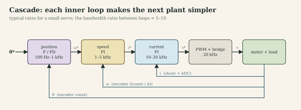
| Loop | Controls | Plant it sees | What it physically changes | Typical rate |
|---|---|---|---|---|
| Current | winding current | $1/(Ls+R)$ with back-EMF disturbance | turns voltage source into torque source; limits current | 10-20 kHz |
| Speed | rotor speed | $k_t/(Js+b)$ | adds damping and rejects load torque | 1-5 kHz |
| Position | rotor angle | $1/s$ (closed speed loop) | adds stiffness; tracks trajectories | 0.1-1 kHz |
Advantages of cascading: each loop can be limited separately (current limit = torque limit, speed limit), tuned separately, and tested separately. The cost: the outer loop bandwidth is limited by the inner ones, and the speed estimate must be good enough for the speed loop.
G.6 Servo control: trajectories and feedforward
Feedback alone reacts to errors after they occur. For a servo task (tracking a moving reference), MF2007’s model-following concept adds two pieces:
- Trajectory planner producing a reference that respects actuator limits: for a trapezoidal velocity profile with acceleration limit $a_{\max}$ and speed limit $v_{\max}$, the reference accelerates for $v_{\max}/a_{\max}$, cruises and decelerates. My group’s planner used 500 rad/s² and 210 rad/s, chosen from the identified model so that the voltage would not saturate.
- Feedforward that inverts the plant model along the trajectory: with current command,
so feedback only has to correct model errors and disturbances. The trajectory must be differentiable as many times as the plant order (twice for position with current input), which is why S-curves (jerk-limited) are used where vibration matters.
G.7 State feedback and LQR
State feedback and pole placement. With full state $x$, $u=-Kx+k_rr$ places all closed-loop poles (the system is controllable, D.7). For the speed-plus-current model $x=[i,\omega]^\top$, $K=[k_i\ k_\omega]$: current feedback adds electrical damping, speed feedback adds mechanical damping and stiffness against load.
LQR chooses $K$ by minimizing $\int(x^\top Qx+u^\top Ru)\,dt$ (derivation in the adaptive and optimal control note). Bryson’s rule sets $Q_{ii}=1/x_{i,\max}^2$, $R=1/u_{\max}^2$. Worked example (nutrunner motor side, current input): $x=[\theta,\omega]^\top$, $J=6.2\cdot10^{-6}$ kg·m², $\theta_{\max}=0.1$ rad, $\omega_{\max}=100$ rad/s, $i_{\max}=1.4$ A (the continuous rating) gives
\[K=[\,14\ \text{A/rad},\ \ 0.064\ \text{A·s/rad}\,],\qquad s_{1,2}=-227\pm216j\ \ (|s|=313\ \text{rad/s},\ \zeta=0.72).\]The Riccati solution automatically produces about 0.7 damping, a typical LQR property. Discretized at $T_s=1$ ms (discrete Riccati equation) the gains become $[11.2,\ 0.057]$ and the poles $z=0.78\pm0.17j$.
Estimation. State feedback needs the full state, but a drive measures angle and current at best. Observers, Kalman filters and their combination with LQR (LQG) are the subject of Part H.
G.8 Robustness: what feedback cannot do
With the 2-DOF polynomial structure, the sensitivity $S=AR/(A_mA_o)$ (model error and disturbance to output) and complementary sensitivity $T=BS/(A_mA_o)$ (sensor noise to output) satisfy
\[S(s)+T(s)=1 .\]At any frequency, you cannot be insensitive to both model error and sensor noise.
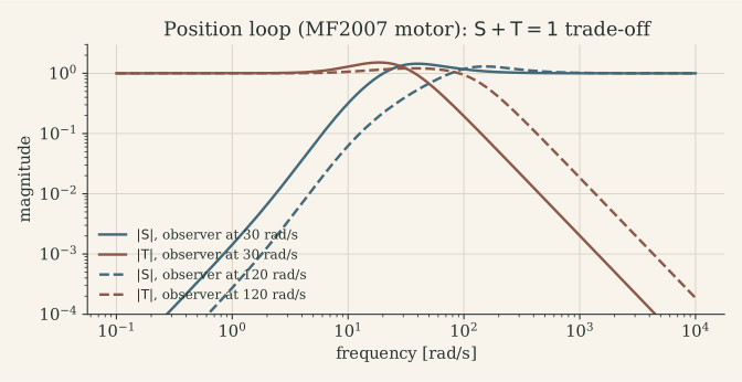
My Workshop B conclusion was the same: slower observer poles reject sensor noise, faster ones reject model error. In a drive the choice is concrete: encoder quantization and current-sensor noise live at high frequency, inertia and friction uncertainty at low frequency.
G.9 From continuous to discrete time
Zero-order hold and exact discretization. A DAC or PWM holds $u$ constant over each sampling interval. The exact discrete model of $\dot x=Ax+Bu$ under ZOH is
\[x_{k+1}=A_dx_k+B_du_k,\qquad A_d=e^{AT_s},\qquad B_d=\int_0^{T_s}e^{A\eta}\,d\eta\,B,\]computed together as the matrix exponential of \(\begin{bmatrix}A&B\\0&0\end{bmatrix}T_s\). For the reduced motor model $\beta/(s+\alpha)$: $\omega_{k+1}=e^{-\alpha T_s}\omega_k+\tfrac{\beta}{\alpha}(1-e^{-\alpha T_s})V_k$.
Two design routes.
- Emulation: design in continuous time, discretize the controller (Tustin $s\approx\frac{2}{T_s}\frac{z-1}{z+1}$ preserves stability; forward Euler does not). Works when $T_s$ is small relative to the closed-loop dynamics.
- Direct digital design: discretize the plant with ZOH and place poles in the $z$-plane ($z=e^{sT_s}$). Accounts for the hold and the sampling exactly and tolerates longer $T_s$. In MF2007, the directly designed position controller worked at $T_s=50$ ms where the emulated one failed.
What sampling costs. The hold delays the signal by $T_s/2$, the computation by up to one more period, and the sampler folds high-frequency content into the band. Part F treats sampling, aliasing, cut-off frequencies, the ADC and PWM; G.10 turns them into a sampling rate for every loop; G.11 handles the actuator limits every real loop hits.
Finite precision. At high sampling rates, poles crowd near $z=1$ ($e^{-\alpha T_s}\approx1-\alpha T_s$) and coefficients need many significant digits. Delta-operator forms, double precision for slow integrators, or fixed-point formats with enough fractional bits avoid this (Part K.5).
Implementation pattern (MF2007 C6). Minimize the latency from sample to actuation by splitting the controller into an output part and an update part:
/* R(z)u = T(z)r - S(z)y, second order, called from the sampling interrupt */
static float u1, u2, r1, r2, y1, y2;          /* controller memory (static!) */

void control_step(float r, float y)
{
    float u = 1.35f*u1 - 0.35f*u2 + 0.65f*r - 0.82f*r1 + 0.27f*r2
              - 10.9f*y + 20.0f*y1 - 9.0f*y2;  /* 1. compute               */
    u = saturate(u, -U_MAX, U_MAX);            /* 2. limit                 */
    write_actuator(u);                         /* 3. write as early as possible */
    u2 = u1; u1 = u;                           /* 4. update memory after   */
    r2 = r1; r1 = r;   y2 = y1; y1 = y;
}
Better still, precompute every term that does not depend on the new sample during the previous period, so only $u=t+d_1r+d_2y$ remains between reading and writing.
G.10 Choosing every sampling frequency in the drive
The lower bound comes from delay. A sampled loop delays the signal by the hold ($T_s/2$, Part F.4), by the computation (from the sampling instant to the output write, up to one full $T_s$ if the output is written at the next tick) and by any filters. The phase lost at the crossover frequency $f_c$ is
\[\Delta\varphi=360°\cdot f_c\,\tau_d .\]| Delay $\tau_d$ | $f_s/f_c$ = 10 | 20 | 30 |
|---|---|---|---|
| hold only, output written immediately ($T_s/2$) | 18° | 9° | 6° |
| hold + one-sample computation delay ($1.5\,T_s$) | 54° | 27° | 18° |
This table is where the rules of thumb come from. Ten to thirty samples per crossover period keep the hold’s phase loss at 6-18°; the implementation pattern of G.9 (write the output as early as possible) decides which row applies. The rules:
| Rule | Source | What it protects |
|---|---|---|
| $\omega_s\in[10,30]\,\omega_b$, $\omega_b$ the fastest of plant, controller and closed loop | MF2007 C4 | phase margin against hold and computation delay |
| 4-10 samples per rise time | MF2007 C4 | the same rule in the time domain |
| $f_s>2f_{\max}$ (Nyquist) | Shannon | necessary, never sufficient for control |
| anti-alias bandwidth $\omega_a\in[0.2,0.33]\,\omega_s$ | MF2007 C4 | aliasing, with a known lag |
| $10\,T_{\text{PWM}}<\tau_e$ | MF2030 | current ripple per PWM period |
| current sampled once per PWM period (or every second), at a fixed phase | drive practice | ripple-free average current (F.1) |
| bandwidth ratio 5-10 between nested loops | cascade design (G.5) | each loop sees the inner one as ideal |
The upper bound comes from cost. Sampling faster is not free:
- CPU load grows as WCET/$T_s$ (Part M.3);
- the M-method speed quantum $2\pi/(N_{\text{cpr}}T_s)$ grows (Part E.5);
- discrete poles crowd toward $z=1$, so coefficients need more precision (G.9);
- noise bandwidth grows, which hurts derivative action most;
- communication and logging bandwidth grow.
Worked numbers from my three set-ups.
- MF2007 speed loop. $\omega_b=24.3$ rad/s, so $\omega_s\in[243,729]$ rad/s and $T_s\in[8.6,26]$ ms. The group ran 2 ms, four to thirteen times faster than necessary. The figure below shows 20 ms is still acceptable, and 50 ms with a one-sample delay overshoots 54 %. Position loop. The observer polynomial (30 rad/s; the report quotes 36 rad/s as the fastest frequency) asks for 6-17 ms with emulation. A controller designed directly in discrete time worked at 50 ms.
- MF2103. The coreless motor’s mechanical time constant is 8.2 ms (a pole at 122 rad/s, 19 Hz). The assignment’s 50 ms period ($\omega_s=126$ rad/s) is slower than the motor itself, so by the 10-30 rule the closed loop can be no faster than 4-13 rad/s (below 2 Hz). At that rate the submitted PI (integral time 9 ms) is dominated by its integral term: every period, the integral adds $t/\tau\approx5.6$ times the value of the proportional term. It overshoots 12 % after reversals at 50 ms, and less at 10 ms (project page).
- A drive with all loops (the architecture of Part N.7: PWM 20 kHz, current 10 kHz, speed 1 kHz, position 100 Hz):
| Loop | Rate | Bandwidth | $f_s/f_c$ | Phase cost, $T_s/2$ | Phase cost, $1.5T_s$ |
|---|---|---|---|---|---|
| Current | 10 kHz (every second PWM period) | 1 kHz | 10 | 18° | 54° |
| Speed | 1 kHz (every 10th current sample) | 50 Hz | 20 | 9° | 27° |
| Position | 100 Hz (every 10th speed sample) | 5 Hz | 20 | 9° | 27° |
| Communication, logging | asynchronous | – | – | – | – |
The current loop sits at the lower end of the rule. Either the one-sample delay is included in its design (direct discrete design), or its bandwidth is lowered to about 600 Hz. The rates are integer ratios of the PWM frequency, so every loop is phase-locked to the switching and to the others (Part M.5). Independent timers at “almost” the same rates drift against each other and produce beat frequencies, as in the aliasing table of F.1.
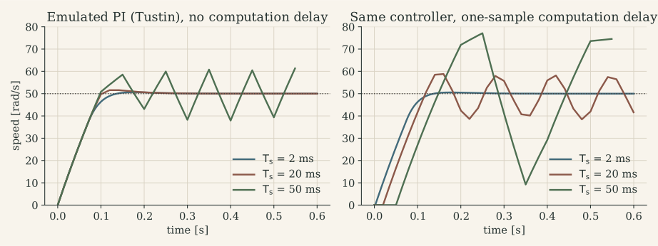
G.11 Saturation and anti-windup
Why windup happens. Every actuator has limits: the bridge cannot apply more than $\pm V_{\text{bus}}$, and the current loop must not exceed $i_{\max}$. While the output is saturated the loop is effectively open: the plant receives $u_{\text{sat}}$ whatever the controller computes. The integrator, however, is a state of the controller with no physical counterpart, and it keeps integrating the error at rate $K_ie$. When the error finally changes sign, the output stays saturated until the integrator has been integrated back down. The result is a large overshoot whose size grows with the area of error accumulated during saturation. Saturation comes from:
- large reference steps;
- large disturbances (a rotor held by hand, a bolt reaching snug);
- wrong initial conditions;
- in a cascade, the inner loop’s limit, which the outer loop sees as saturation.
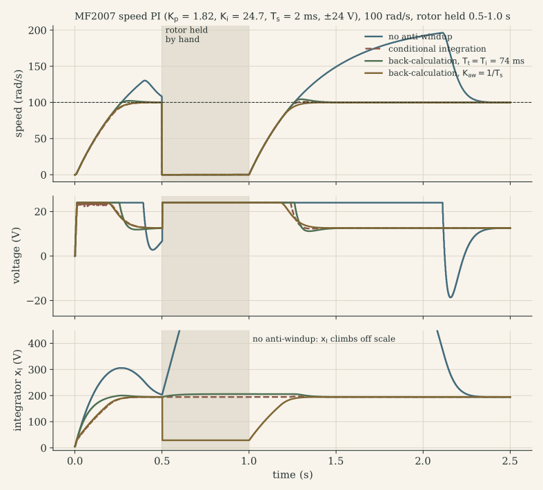
The simulation reproduces the experiment the MF2007 workshop did by hand: stopping the motor under a speed reference and letting go.
Method 1: conditional integration (clamping). Integrate only when it helps: stop integrating while the output is saturated and the error would push it further into saturation.
float v = KP*e + xi;                              /* unsaturated output  */
float u = fminf(fmaxf(v, -UMAX), UMAX);
if (u == v || e*v < 0.0f) xi += TS*KI*e;          /* integrate unless it winds up */
Method 2: back-calculation (tracking). Feed the difference between the saturated and the unsaturated output back into the integrator through a tracking time constant $T_t$ (MF2007 C3):
\[x_{I,k+1}=x_{I,k}+T_s\Big[K_ie_k+\frac{1}{T_t}\,(u_{\text{sat},k}-v_k)\Big].\]When the output is not saturated the extra term is zero. When it is, the integrator is pulled toward the value at which the output just touches the limit, with time constant $T_t$. Åström and Hägglund suggest a $T_t$ between the derivative and the integral time. For a PI, $T_t=T_i=K_p/K_i$ is a common start (74 ms for the MF2007 loop, 4 % overshoot in the figure).
The deadbeat special case. With $T_t=T_s$ (MF2007’s $K_{\text{aw}}=1/T_s=500$), the update becomes $x_{I,k+1}=u_{\text{sat},k}-K_pe_k+T_sK_ie_k$. The integrator is placed in one step exactly where the unsaturated output equals the limit. Recovery is the fastest possible (0 % overshoot in the figure). The price is sensitivity to noise near the limit, because the output can chatter in and out of saturation.
Method 3: incremental (velocity) form. Compute the change of output and store the saturated result:
\[u_k=\operatorname{sat}\big(u_{k-1}+q_0e_k+q_1e_{k-1}\big).\]The stored state is the actual actuator command, so there is nothing to wind up. My final MF2103 controller has this form. It must still be protected against arithmetic overflow, as discussed below.
Method 4: anti-windup for polynomial (RST) controllers. A general controller $R(q)u=T(q)r-S(q)y$ has its integrator hidden in $R$, and a 2-DOF structure can contain two integrators (in the reference and in the feedback path) that wind up separately. MF2007’s advice is to merge them into one block. Åström and Wittenmark’s observer form does this: choose a stable monic polynomial $A_o$ of the same degree as $R$ (the observer polynomial is the natural choice) and implement
\[A_o(q)\,u=T(q)\,r-S(q)\,y+\big(A_o(q)-R(q)\big)\,v,\qquad v=\operatorname{sat}(u).\]Without saturation ($v=u$) this is the original controller. With saturation, the controller’s internal states evolve with the stable dynamics of $A_o$, driven by the input the plant actually received.
Windup in cascades. When the speed PI’s output (the current reference) is clamped at $i_{\max}$, the speed integrator must see that clamp, by back-calculation on $i^\ast$. When the current loop itself runs out of voltage (high speed, a sagging battery), the actual current stays below its reference, and the speed integrator winds up unless it is told. Either pass a “saturated” flag up the cascade, or back-calculate the speed integrator on the measured current. The cleanest anti-windup is not to saturate at all. MF2007’s trajectory planner (G.6) chose 500 rad/s² and 210 rad/s so that the voltage never reached its limit.
Windup meets fixed point: the two MF2103 controllers. Integer controllers add a second failure mode, overflow: windup makes a state large, and overflow makes it wrap around to the opposite sign.
- RTOS version (positional, back-calculation).
Iaccumulates error·ms and contributeski*Ito the output. The deadbeat correction would be $(u-v)/k_i$. The code adds(u - v)*kantwithkant = 300, which is $k_i\cdot k_{\text{ant}}=9\cdot10^5$ times stronger. In the replay with the rotor held, the unsaturated output already exceeds 32 bits ($2.16\cdot10^9$) before the clamp, and the correction product ($1.4\cdot10^8\times300$) is 19 times larger than anint32_tcan hold: 77 overflow events (Part K.6). - Final super-loop version (incremental). The output is clamped at $\pm2\cdot10^9$, but the clamp comes after the addition, and only $2^{31}-2\cdot10^9=1.47\cdot10^8$ of headroom remains. At 10 ms one increment at full error is $3.3\cdot10^7$, which fits. At 50 ms it is $1.56\cdot10^8$, which does not. In the replay with the rotor held at 50 ms, the sum wraps to a large negative number and the clamp turns it into full reverse duty while the rotor is held.
The fixes are the same in both cases: compute the sum in int64_t (or float) and clamp before storing, keep the limits well inside the type’s range, and test the stalled-rotor case, not just the step response.
G.12 What changes on a microcontroller
| In simulation | On the MCU |
|---|---|
| continuous signals | samples at $T_s$, held by ZOH |
| zero computation time | latency from sample to write, possibly variable (jitter) |
| exact derivative of position | difference quotient on quantized counts |
| infinite resolution | ADC, encoder and PWM quantization |
| real numbers | float (with or without FPU) or fixed point |
| ideal actuator | voltage saturation, dead time, current limit |
| one task | ISRs and threads competing for the CPU |
| sensors without delay | filter lag, conversion time, communication latency |
The emulated PI of G.10 and the timing results in Part M show that the last three rows usually dominate.
What to remember
- Current loop: PI with zero at $R/L$, $K_p=\omega_cL$, $K_i=\omega_cR$; it turns the motor into a torque source.
- Speed and position PI/PID by pole placement on the reduced plant; cascade from the inside out with a 5-10× bandwidth ratio; trajectory planning and feedforward for servo tasks.
- LQR gives well-damped state feedback; the state it needs comes from an estimator (Part H).
- $S+T=1$: no loop is insensitive to both model error and sensor noise at the same frequency.
- Sample 10-30× faster than the fastest closed-loop frequency: the hold costs $180°\cdot f_c/f_s$, a one-sample computation delay three times that; run all loops at integer ratios of the PWM frequency.
- Every loop saturates: use conditional integration, back-calculation ($T_t\approx T_i$, or $T_s$ for deadbeat recovery) or the incremental form; merge the integrators of RST controllers; in fixed point, clamp before the value can overflow.
Part H. Estimation and sensor fusion
Every sensor of Part E measures something slightly different from what the controller needs, with noise, quantization, bias and delay. Estimation combines these imperfect measurements with a model of the motor to produce the best available value of the state; when several sensors are combined, it is called sensor fusion. Three situations occur in every drive:
- A state is not measured at all: speed (from a position sensor), load torque, rotor angle in a sensorless motor.
- A state is measured, but too coarsely or noisily: the quantized speed of E.5.
- Two sensors measure related quantities with complementary errors: a motor-side and a load-side encoder; current-based torque and a torque transducer; an encoder and an accelerometer.
H.1 The model as a sensor
The central idea is predict, then correct. A model driven by the known input predicts the state; the measurement corrects the prediction:
\[\hat x_k^-=A_d\hat x_{k-1}+B_du_{k-1},\qquad \hat x_k=\hat x_k^-+L\,(y_k-C\hat x_k^-).\]With a perfect model, one measurement would be enough to initialize it; with a perfect, complete measurement, no model would be needed. The gain $L$ sets the balance between trusting the model and trusting the sensor. In a motor drive the model’s input is the current or voltage the controller itself commands, so the controller is a sensor of torque. That is why model-based estimators can see through encoder quantization without the lag of a filter.
Observability (Part D.7) decides what can be estimated. With the angle measured, the speed and a constant load torque are observable. With only the speed measured, the absolute angle is not. With only the current measured, speed is observable through the back-EMF, which is the basis of sensorless control (H.6).
H.2 Luenberger observers and disturbance observers
The observer. With $\hat x_{k+1}=A_d\hat x_k+B_du_k+L(y_k-C\hat x_k)$, the estimation error obeys $e_{k+1}=(A_d-LC)\,e_k$. Its poles are placed by choosing $L$, typically 2-5 times faster than the controller’s: fast enough that the controller sees a converged estimate, slow enough not to amplify sensor noise. The observer polynomial $A_o$ in MF2007’s polynomial design (G.4) is exactly this choice. Figure G.8 shows its trade-off: observer poles at 120 rad/s instead of 30 rad/s lower the peak sensitivity from 1.44 to 1.30 but transmit about ten times more sensor noise at 1000 rad/s.
The disturbance observer. Add the load torque as a state that is assumed constant between samples:
\[\dot\theta=\omega,\qquad J\dot\omega=k_ti-\tau_L,\qquad \dot\tau_L=0 .\]With the angle measured, the observer estimates $\hat\tau_L$, which collects friction, load and model error. Feeding it forward, $i_{\text{ff}}=\hat\tau_L/k_t$, lets the speed loop reject load torque as fast as the observer converges, with less reliance on the integrator. This is the internal model principle in observer form: a constant-disturbance model gives integral action. Drives use it to compensate friction and cogging, and a tightening tool could use $\hat\tau_L$ as a model-based torque estimate alongside its transducer.
H.3 The Kalman filter
The Kalman filter is the observer whose gain is optimal for a stated noise model. It assumes
\[x_{k+1}=A_dx_k+B_du_k+w_k,\qquad y_k=Cx_k+v_k,\qquad w\sim\mathcal N(0,Q),\ \ v\sim\mathcal N(0,R).\]| Step | Equations | Meaning |
|---|---|---|
| Predict | $\hat x^-=A_d\hat x+B_du$, $\ P^-=A_dPA_d^\top+Q$ | the model moves the estimate; uncertainty grows by $Q$ |
| Gain | $K=P^-C^\top(CP^-C^\top+R)^{-1}$ | trust the sensor in proportion to the model’s uncertainty |
| Update | $\hat x=\hat x^-+K(y-C\hat x^-)$, $\ P=(I-KC)P^-$ | the measurement shrinks the uncertainty |
What Q and R mean in a drive. $R$ is the sensor noise. For an encoder it is the quantization variance $\Delta^2/12$ with $\Delta=2\pi/N_{\text{cpr}}$, valid when the motion spans several counts between samples. $Q$ is how much the motor departs from the model between samples: unmodelled torques (friction changes, cogging, load steps) and current-measurement errors. Only the ratio of $Q$ to $R$ shapes the gain. For a time-invariant model, $P$ and $K$ converge to constants given by the discrete algebraic Riccati equation. A microcontroller runs only the constant-gain observer, computed offline, with no matrix inversion at run time.
A first example. Take a 4096-count encoder, $T_s=1$ ms, the nutrunner’s motor-side inertia ($6.2\cdot10^{-6}$ kg·m²) and an unknown torque with a standard deviation of 0.2 mN·m per sample. The steady-state gain is $L=[0.32,\ 60.2]$. The posterior speed standard deviation is 0.07 rad/s, against a quantum of 1.53 rad/s (standard deviation 0.63 rad/s) for naive count differencing.
Fusion example on the MF2103 motor. The figure compares four estimators on the same simulated data: 2048 counts/rev, 1 kHz, the MF2103 coreless motor with an ideal speed loop, an unknown 0.4 mN·m load step at 0.45 s, then a slow-down to 20 rpm. The Kalman filter’s state is $[\theta,\omega,\tau_L]$ and it uses the encoder counts and the measured current.
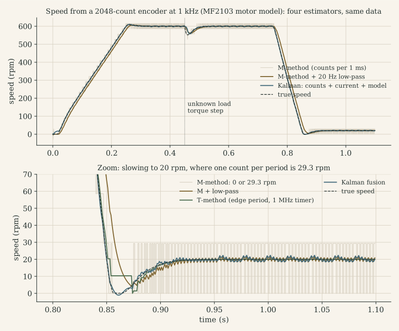
| RMS speed error (rpm) | M-method | M + 20 Hz low-pass | T-method | Kalman |
|---|---|---|---|---|
| cruise at 600 rpm | 14.6 | 1.1 | 4.5 | 1.4 |
| 150 ms after the load step | 13.5 | 7.6 | 4.1 | 7.9 |
| at 20 rpm | 13.7 | 1.2 | 0.07 | 1.1 |
| mean error on the 0→600 rpm ramp | – | −19 | – | 0.1 |
The Kalman filter’s load-torque estimate converges to 0.688 mN·m; the true value, including Coulomb friction, is 0.685 mN·m. The reaction to the step depends on $Q$, which encodes how fast the load torque is believed to change. That is a tuning decision, not a free lunch:
| Load-torque noise $q_\tau$ per step | Cruise error | Error after the load step |
|---|---|---|
| $2\cdot10^{-5}$ N·m | 2.0 rpm | 4.3 rpm |
| $5\cdot10^{-6}$ N·m (figure) | 1.4 rpm | 7.9 rpm |
| $2\cdot10^{-6}$ N·m | 0.9 rpm | 12.9 rpm |
Each method wins somewhere. A practical drive fuses them: M/T edge timing as the measurement at low speed, the model with the current input for dynamics, and a load-torque state for disturbances. The filter is only as good as its model. If $J$ or $k_t$ is wrong, the prediction is biased and the estimate lags or overshoots on every acceleration, which is why identification (Part D.8) comes before estimation.
H.4 Complementary filters: fusing two sensors
When two sensors measure the same quantity, one accurate at low frequency (and noisy or delayed at high frequency) and the other the opposite, combine them with complementary filters:
\[\hat x=F(s)\,y_{\text{LF}}+\big(1-F(s)\big)\,y_{\text{HF}},\qquad F(s)=\frac{1}{\tau s+1}.\]Because $F+(1-F)=1$, the true signal passes without gain or phase error, while each sensor’s noise is suppressed in the band where that sensor is bad. The crossover $1/\tau$ belongs where the two noise spectra cross. Often the high-frequency sensor measures a rate, which is integrated: $\hat x=F\,y_{\text{LF}}+(1-F)\,\tfrac1s\dot y_{\text{HF}}$. In discrete time,
\[\hat x_k=\alpha\,(\hat x_{k-1}+T_s\,\dot y_{\text{HF},k})+(1-\alpha)\,y_{\text{LF},k},\qquad \alpha=\frac{\tau}{\tau+T_s}.\]In motor drives:
| Low-frequency sensor | High-frequency sensor | Fused estimate | Why |
|---|---|---|---|
| encoder speed (quantized, lagging) | acceleration from current, $(k_ti-\hat\tau_L)/J$ | speed | the structure the Kalman filter of H.3 finds by itself |
| load-side encoder (true output angle, behind gear compliance) | motor-side encoder divided by $n$ (fast, sees backlash) | output angle | dual-loop position control in machine tools: accuracy from the load, stability from the motor |
| torque transducer (accurate, filtered) | $\eta nk_ti$ (fast, gearbox efficiency uncertain) | output torque | fast torque shut-off without losing calibration |
| accelerometer tilt (noisy, unbiased) | gyroscope (smooth, drifting) | attitude | the classic IMU case, same mathematics |
A steady-state Kalman filter for two sensors with these noise characteristics is a complementary filter, with the crossover set by the noise ratio. The complementary form is the one to implement first: one parameter, no model of the plant needed, and easy to reason about.
H.5 Tracking loops: the PLL as a speed observer
Resolvers, sin/cos encoders and sensorless back-EMF estimates deliver an angle, often only as $\sin\theta$ and $\cos\theta$. A tracking loop (phase-locked loop) extracts angle and speed from them:
\[\varepsilon=\sin\theta\cos\hat\theta-\cos\theta\sin\hat\theta=\sin(\theta-\hat\theta)\approx\theta-\hat\theta,\qquad \hat\omega=K_p\varepsilon+K_i\!\int\!\varepsilon\,dt,\qquad \dot{\hat\theta}=\hat\omega .\]Linearized, $\hat\theta/\theta=(K_ps+K_i)/(s^2+K_ps+K_i)$: a second-order filter with $\omega_n=\sqrt{K_i}$ and $\zeta=K_p/(2\sqrt{K_i})$. It is a type-2 loop: no error at constant speed, and a constant lag $\alpha/K_i$ at constant acceleration $\alpha$. For a 50 Hz tracking bandwidth ($K_i=9.87\cdot10^4$ s⁻², $K_p=444$ s⁻¹, $\zeta=0.71$) and the 251 rad/s² ramp of the figure in H.3, the lag is 2.5 mrad, about one encoder count. The PLL is an observer without an input model: it assumes constant speed. Adding $k_ti/J$ as feedforward into its integrator turns it into the disturbance observer of H.2.
H.6 Sensorless control: estimation from electrical measurements
Without a position sensor, angle and speed are estimated from the motor’s own voltages and currents:
- DC motor: $\hat\omega=(v-R\,i)/k_e$, the simplest estimator. It is noisy (PWM, the neglected $L\,di/dt$) and biased by $R$, which rises 0.39 %/K with temperature.
- PM synchronous motor: the back-EMF in the stationary frame, $e_{\alpha\beta}=\omega\psi_m[-\sin\theta_e,\ \cos\theta_e]^\top$, is estimated as $\hat e=v-Ri-L\,di/dt$, and a PLL (H.5) extracts $\theta_e$ and $\omega$. Flux observers integrate $v-Ri$ instead.
- Limits: the back-EMF vanishes at standstill, and at low speed the voltage errors of the inverter (dead time, F.4) and of $R$ dominate. These methods therefore work above roughly 5-10 % of rated speed. Salient machines ($L_d\ne L_q$) can be tracked at standstill by high-frequency injection. Surface-magnet BLDC motors have little saliency and start open-loop (current ramp, “I/f”) before switching to the estimator. The fusion with the winding temperature of E.4 corrects $R$.
H.7 LQG: optimal control with an optimal estimate
LQG is LQR (Part G.7) applied to the Kalman estimate. The separation principle guarantees that the closed-loop poles are the union of the controller’s and the estimator’s, so the two can be designed independently. It guarantees nothing about robustness: LQG can have arbitrarily small stability margins (Doyle, 1978). In practice, check the margins of the combined loop and detune the estimator if needed (loop-transfer recovery is the systematic version).
| PID / PI cascade | LQR (state feedback) | LQG (LQR + Kalman) | |
|---|---|---|---|
| Needs | output measurements | full state | model + noise models |
| Tuning knobs | gains, bandwidths | weights $Q$, $R$ | $Q$, $R$, noise intensities |
| Multivariable | loop by loop | natively | natively |
| Constraints | clamps + anti-windup | not native (MPC instead) | not native |
| Robustness | margins easy to read | good margins (state feedback) | no guaranteed margins |
| Typical place in a drive | current and speed loops | position/vibration control | speed estimation, sensor fusion |
H.8 Estimation in firmware: practical rules
- Align in time. Fuse measurements taken at the same instant. Trigger the encoder read and the ADC from the same PWM event (Part M.5). If a measurement arrives late, as over CAN or TCP, propagate the estimate to the measurement’s timestamp or model the delay. In MF2103’s distributed version, the server’s speed value is at least one network delay old.
- Fix the rate. Gains are computed for one $T_s$; sampling jitter (Part M.4) acts as model error.
- Watch the innovations. $y-C\hat x^-$ should be zero-mean and white. A bias reveals a model error (wrong $k_t$, unmodelled friction); correlation reveals wrong $Q/R$.
- Bound and reset. Clamp estimated states to physical limits (a load torque cannot exceed stall torque). Re-initialize after encoder errors (at the index pulse) and handle the friction sign change at reversals.
- Grow the estimator in steps. M/T speed with a first-order filter; then a disturbance observer; then a Kalman filter once the model and the noise have been identified.
What to remember
- Estimation = predict with a model driven by the known input, correct with the measurement; the gain sets the trust between them.
- Observers place the error poles 2-5× faster than the controller; a disturbance observer estimates load torque and gives integral action by feedforward.
- The Kalman filter makes the gain optimal for stated noise: $R$ from the sensor (quantization $\Delta^2/12$), $Q$ from what the model misses; it runs as a constant-gain observer.
- Complementary filters fuse a low-frequency-accurate sensor with a high-frequency-accurate one without distorting the signal.
- PLLs extract angle and speed from resolvers, sin/cos encoders and back-EMF; sensorless estimation fails near standstill without saliency.
- LQG separates design but not robustness: check margins.
Part I. BLDC and PMSM modelling and control
I.1 Three-phase quantities
A star-connected three-phase winding has phase voltages $v_a,v_b,v_c$ measured to the star point (usually not accessible), phase currents $i_a,i_b,i_c$ equal to the line currents, and line-to-line voltages $v_{ab}=v_a-v_b$ that can be measured at the terminals. Kirchhoff at the star point gives $i_a+i_b+i_c=0$, so two currents determine the third: drives measure two (or reconstruct from one DC-link shunt).
Per phase:
\[v_x=R\,i_x+L\frac{di_x}{dt}+e_x(\theta_e)+v_n,\]with $L=L_{\text{self}}-M$ for a balanced winding, $e_x$ the back-EMF of phase $x$ as a function of electrical angle, and $v_n$ the star-point voltage relative to the inverter’s reference. The torque is the electrical power converted, divided by mechanical speed:
\[\tau=\frac{e_ai_a+e_bi_b+e_ci_c}{\omega_m}.\]Sizing example (MF2030). A 6-pole PMSM must give 2 N·m at 3000 rpm with $k_{T,\text{rms}}=0.96$ N·m/A, $R_{ll}=15.5$ Ω, $L_{ll}=30$ mH, $k_{E}=58$ V per 1000 rpm (line, RMS). Current: $2/0.96=2.1$ A RMS. Electrical frequency: 50 Hz mechanical × 3 pole pairs = 150 Hz. Per-phase voltage drops: $RI=16$ V, $\omega_eLI=29.5$ V, back-EMF $174/\sqrt3=100$ V. With current in phase with back-EMF, $U_{ph}=\sqrt{(100+16)^2+29.5^2}\approx120$ V, i.e. 208 V line-to-line: the supply must exceed this, and the inductive drop grows with speed, so the voltage margin shrinks exactly where it is needed most.
I.2 BLDC six-step commutation
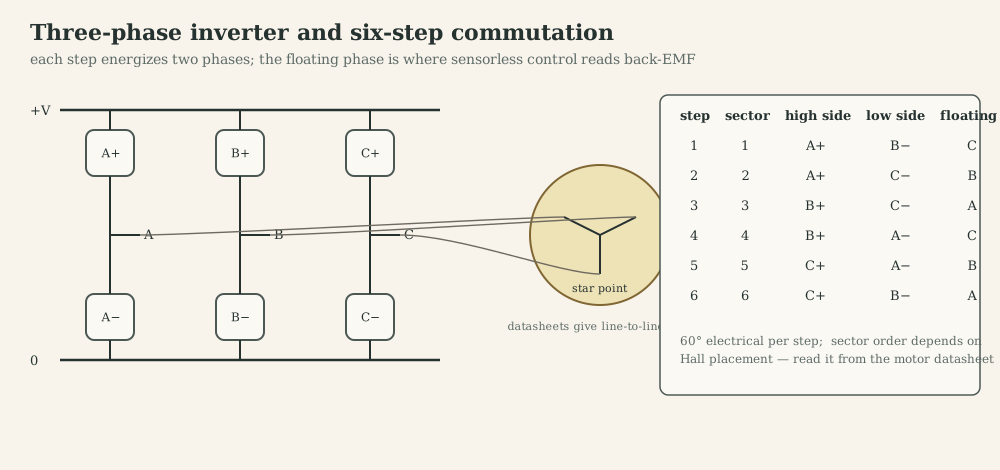
Current path in one step. In step 1 (A+, B−), current flows from the bus through the A high-side switch, into phase A, through the star point, out of phase B and through the B low-side switch to ground. Phase C carries no current and its terminal voltage floats at $v_n+e_c$, which is how sensorless controllers read back-EMF.
PWM in six-step. The bridge applies $D\,V_{dc}$ on average across the two active phases. Common schemes: PWM on the high-side switch with the low side held on (current freewheels through the low-side switch and the opposite low-side body diode during the off-time, slow decay); or complementary PWM on the active leg with synchronous rectification. A single DC-link shunt sees the phase current only during active states, so it is sampled in the middle of the on-time.
Torque ripple. At each commutation the incoming phase current rises at a rate set by $V_{dc}-e$ and the outgoing one decays at a rate set by $e$ (or $V_{dc}+e$ in fast decay). When these differ, the sum, and with it the torque, dips: commutation ripple, worst at low and at high speed.
Sensorless six-step. In the floating phase, the terminal voltage crosses $V_{dc}/2$ (the “virtual neutral”) when its back-EMF crosses zero, 30° electrical before the ideal commutation instant. The controller detects the zero crossing, waits half a sector (estimated from the previous sector time) and commutates. Below roughly 5-10 % of rated speed the back-EMF is too small, so starting needs an open-loop align-and-ramp sequence.
Hardware example: a velocity shield. My Nucleo shield for the BX4 lets the gate driver do the six-step commutation. A DRV8323S in 1×PWM mode reads the three Hall signals, chooses the sector and applies one PWM to the active pair. The MCU only closes the speed loop: it times Hall edges for the speed estimate (the T-method of E.5) and limits the duty with the DC-link current. Design details are on the project page.
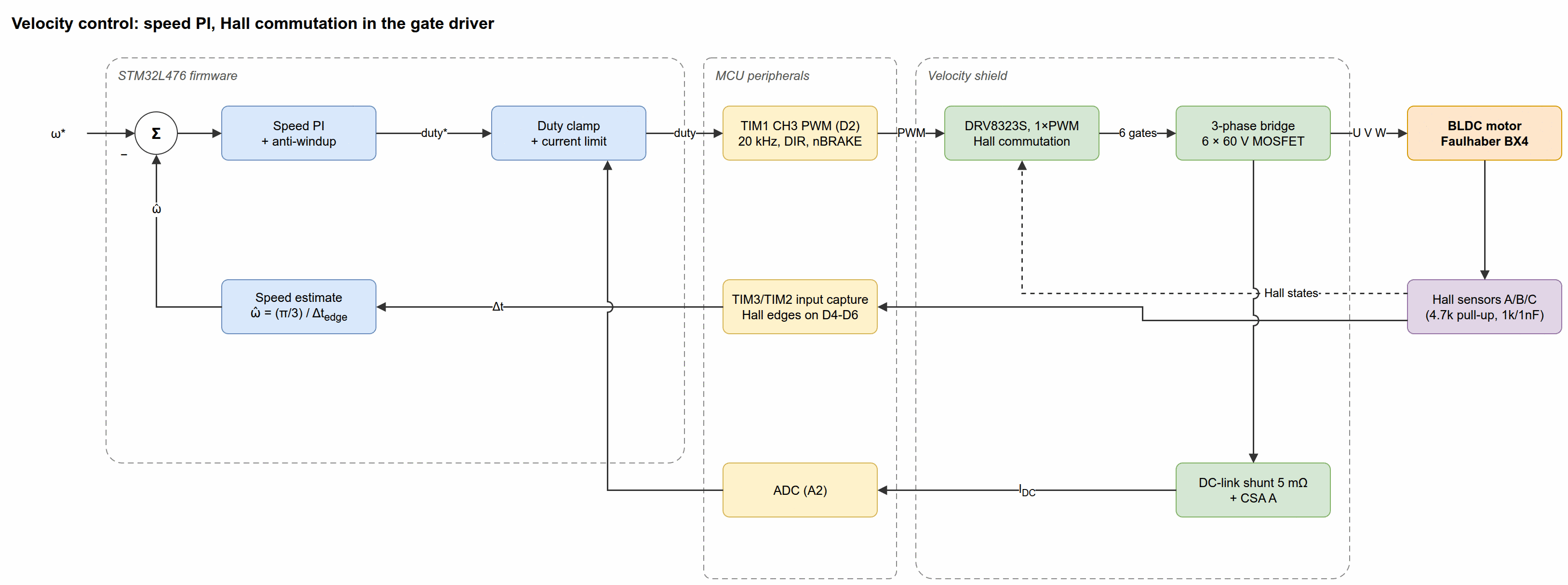
I.3 Sinusoidal commutation and position sensing
A PMSM needs a continuous rotor angle to place current at 90° electrical to the magnet flux.
- Incremental encoder: $N$ lines give $4N$ counts per revolution with quadrature decoding; an index pulse marks one position per revolution. It is relative: the electrical zero must be found at start-up.
- Absolute encoders and resolvers: report angle directly; resolvers are robust analog transformers used in traction and aerospace.
- Hall sensors give six sectors (60° resolution), enough for six-step and for initializing an incremental encoder.
- Sensorless observers estimate $\theta_e$ from voltages and currents (back-EMF observers, PLLs; high-frequency injection at standstill for salient machines).
Encoder alignment. The offset between the encoder count and the magnet’s d-axis is found by injecting a d-axis current (or a fixed voltage vector): the rotor turns until its magnet aligns with the stator field, and that encoder value is the electrical zero. An offset error $\Delta\theta$ reduces torque by $\cos\Delta\theta$ and adds a $\sin\Delta\theta$ component along d; with a 90° error the current produces no torque, and with an error beyond 90° positive feedback can make the motor run away. Always verify alignment by commanding small $i_q$ in both directions and checking that the shaft turns the expected way.
I.4 From abc to αβ to dq
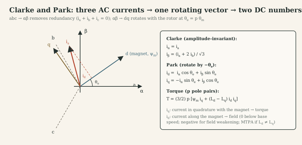
Space vector. Each phase current produces flux along its winding axis ($0°$, $120°$, $240°$). Their sum is one vector,
\[\vec i_s=\tfrac23\big(i_a+i_b\,e^{j2\pi/3}+i_c\,e^{j4\pi/3}\big)=i_\alpha+j\,i_\beta .\]The factor 2/3 makes the transform amplitude-invariant: balanced sinusoidal phase currents of amplitude $I$ give a vector of length $I$. With $i_c=-i_a-i_b$:
\[i_\alpha=i_a,\qquad i_\beta=\frac{i_a+2i_b}{\sqrt3}\qquad\textbf{(Clarke)}.\]Worked example (MF2030). $i_a=7$ A, $i_b=2.6$ A, so $i_c=-9.6$ A: $i_\alpha=7$, $i_\beta=(7+5.2)/\sqrt3=7.04$, so $\vec i_s=9.93$ A at 45°. Projecting back onto the phase axes recovers 7, 2.6 and −9.6 A.
Park. Rotate by the rotor’s electrical angle so that d points along the magnet’s north pole:
\[\begin{bmatrix}i_d\\i_q\end{bmatrix}=\begin{bmatrix}\cos\theta_e&\sin\theta_e\\-\sin\theta_e&\cos\theta_e\end{bmatrix}\begin{bmatrix}i_\alpha\\i_\beta\end{bmatrix}.\]What the transforms accomplish physically. Clarke removes the redundancy of three currents that must sum to zero and gives the direction of the stator’s magnetomotive force. Park looks at that direction from the rotor. When the motor runs at constant torque and speed, the phase currents are AC at $\omega_e$, but $i_d$ and $i_q$ are DC: the AC control problem becomes two DC control problems, one per axis, each like a DC motor.
Voltage equations in dq. Start from the stator-frame vector equation $\vec u_s=R\vec i_s+L\,d\vec i_s/dt+d\vec\psi_m/dt$ with $\vec\psi_m=\psi_me^{j\theta_e}$ (surface magnets, $L_d=L_q=L$). Substitute $\vec i_s=\vec i_{dq}e^{j\theta_e}$ and $\vec u_s=\vec u_{dq}e^{j\theta_e}$; the product rule gives an extra $j\omega_e$ term, and dividing by $e^{j\theta_e}$:
\[\vec u_{dq}=R\vec i_{dq}+L\frac{d\vec i_{dq}}{dt}+j\omega_eL\vec i_{dq}+j\omega_e\psi_m .\]Splitting real and imaginary parts, and allowing $L_d\neq L_q$ for interior magnets:
\[v_d=Ri_d+L_d\frac{di_d}{dt}-\omega_eL_qi_q,\qquad v_q=Ri_q+L_q\frac{di_q}{dt}+\omega_eL_di_d+\omega_e\psi_m .\]The terms $\mp\omega_eLi$ are cross-coupling from the rotation of the frame; $\omega_e\psi_m$ is the back-EMF, appearing only on the q-axis.
Torque. Power balance in dq (with the 3/2 factor that amplitude-invariant transforms require) gives
\[\tau=\tfrac32\,p\,\big[\psi_m\,i_q+(L_d-L_q)\,i_d\,i_q\big].\]Why $i_q$ makes torque and what $i_d$ does. The q-axis is 90° electrical ahead of the magnet: current there sits under the strongest flux, so Lorentz force is maximal (MF2030’s lever analogy: current is the force, flux linkage the lever arm, and the torque is maximal when they are perpendicular). Current along d is parallel to the magnet’s flux: it produces no Lorentz torque, but it strengthens or weakens the air-gap flux. In a surface-PM machine, keep $i_d=0$ for minimum copper loss per torque; use negative $i_d$ to reduce back-EMF at high speed (field weakening); in an interior-PM machine ($L_q>L_d$) a negative $i_d$ also adds reluctance torque (MTPA).
I.5 Field-oriented control
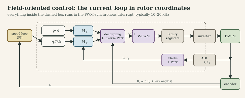
The chain, once per PWM period:
- Sample two phase currents at the PWM centre (Part J.8), read the encoder angle.
- Clarke → $i_\alpha,i_\beta$; Park with $\theta_e=p\theta_m+\theta_{\text{offset}}$ → $i_d,i_q$.
- Two PI controllers: $i_d^\ast=0$ (or field-weakening value), $i_q^\ast=\tau^\ast/(\tfrac32p\psi_m)$ from the speed loop, both clamped.
- Decoupling: add $-\omega_eL_qi_q$ to $v_d^\ast$ and $\omega_eL_di_d+\omega_e\psi_m$ to $v_q^\ast$, so each PI sees only $1/(Ls+R)$.
- Voltage limit: scale $(v_d^\ast,v_q^\ast)$ to the available circle, giving priority to $v_q$ (torque) or $v_d$ (control of field) by design, and back-calculate anti-windup.
- Inverse Park → $v_\alpha,v_\beta$ (using the angle advanced by $1.5\,\omega_eT_s$ to compensate the computation and PWM delay).
- SVPWM → three compare values; load them into the timer’s shadow registers before the next update event.
Each current PI is designed exactly like G.2 on $1/(L_{d,q}s+R)$.
Hardware example: a torque shield. The second shield runs exactly this chain. Three low-side 5 mΩ shunts feed the DRV8323S’s current amplifiers, the ADC is injected at the PWM centre, an encoder in timer encoder mode gives $\theta_e$, and TIM1 produces three centre-aligned PWMs (details on the project page).
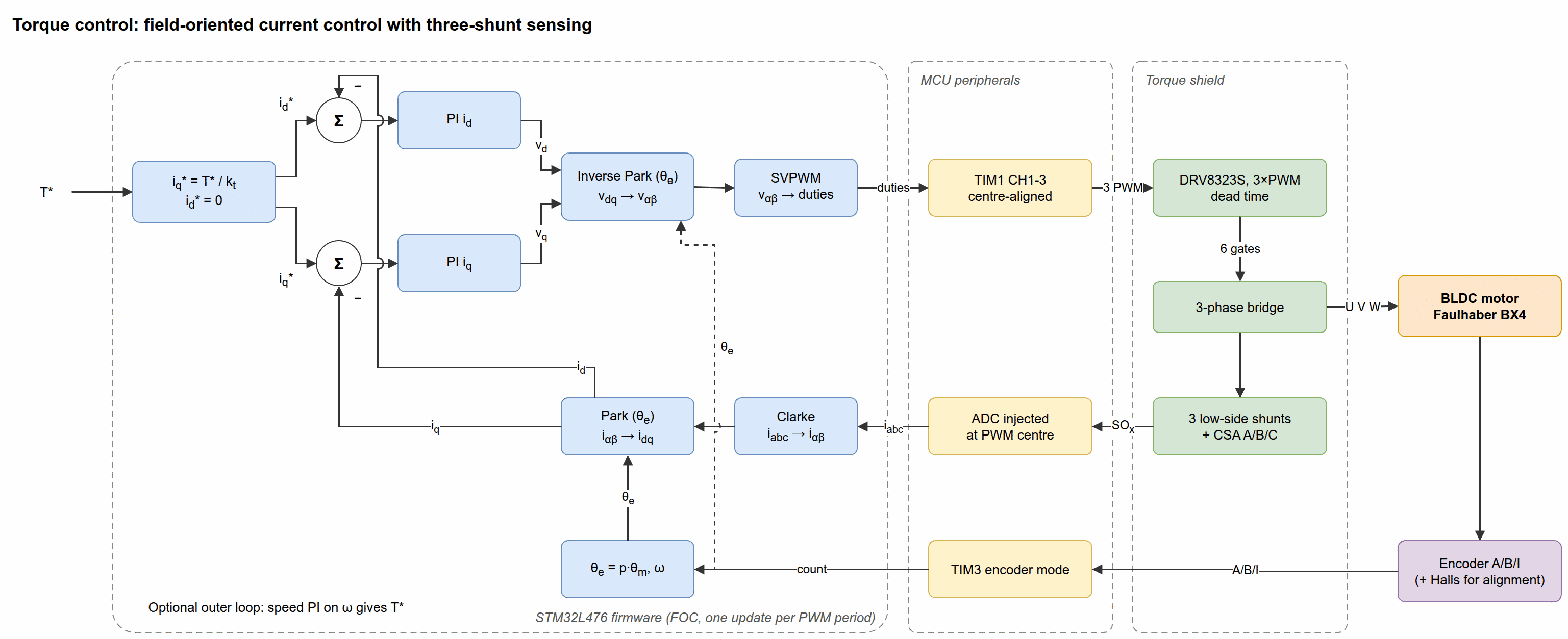
I.6 Space-vector PWM
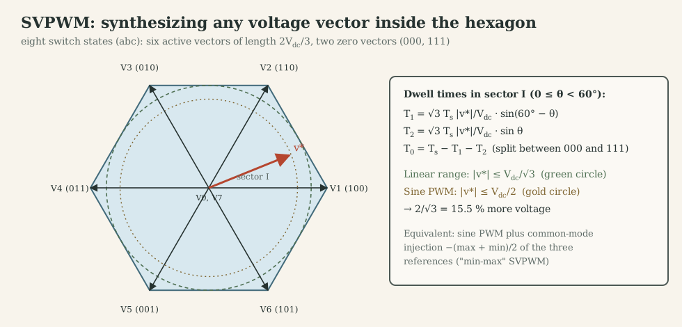
The three-phase inverter has $2^3=8$ switch states. Six give active vectors of length $\tfrac23V_{dc}$ at 60° intervals; two (000, 111) give zero. For a reference vector $v^\ast$ at angle $\theta$ in sector I:
\[T_1=\frac{\sqrt3\,T_s|v^\ast|}{V_{dc}}\sin(60^\circ-\theta),\qquad T_2=\frac{\sqrt3\,T_s|v^\ast|}{V_{dc}}\sin\theta,\qquad T_0=T_s-T_1-T_2 .\]The largest circle that fits inside the hexagon has radius $V_{dc}/\sqrt3$, compared with $V_{dc}/2$ for sine PWM: 15.5 % more usable voltage, which directly raises base speed. An equivalent and easier implementation adds a common-mode offset to sine references:
\[v_x^{\ast\prime}=v_x^\ast-\tfrac12\big(\max(v_a^\ast,v_b^\ast,v_c^\ast)+\min(v_a^\ast,v_b^\ast,v_c^\ast)\big),\]which the star-connected motor cannot see (it only responds to differential voltages). Duty for each leg is then $D_x=\tfrac12+v_x^{\ast\prime}/V_{dc}$.
I.7 Loop design, field weakening and MTPA
Current loops: PI per axis with zero at $R/L$, bandwidth 1-2 kHz for small motors at 20 kHz PWM, limited by sampling delay and voltage margin. Speed loop: as in G.3 with $k_t=\tfrac32p\psi_m$. Position loop: P (or PI) on top of speed, or a state-feedback design.
Voltage and current limits. The inverter limits $\sqrt{v_d^2+v_q^2}\le V_{\max}=V_{dc}/\sqrt3$ (SVPWM linear range); the motor and inverter limit $\sqrt{i_d^2+i_q^2}\le I_{\max}$. In steady state with $R$ neglected and $L_d=L_q=L$,
\[\omega_e\sqrt{(Li_q)^2+(\psi_m+Li_d)^2}\le V_{\max}.\]At low speed the voltage limit is irrelevant (constant-torque region with $i_d=0$). The base speed $\omega_{e,b}=V_{\max}/\sqrt{\psi_m^2+(LI_{\max})^2}$ is where full current and full voltage meet. Above it, negative $i_d$ reduces the term $\psi_m+Li_d$ and allows higher speed at reduced $i_q$ (constant-power region). For interior magnets, MTPA chooses the $(i_d,i_q)$ pair that gives the most torque per ampere, using the reluctance term in the torque equation.
Case-study hook. The Faulhaber BX4 in the nutrunner has $p=2$ and line-to-line $R=1.45$ Ω, $L=110$ µH, so per phase (star) 0.73 Ω and 55 µH. Its flux linkage $\psi_m$ would be measured, as MF2030’s no-load test does, by back-driving the motor and reading the line-to-line back-EMF amplitude: $\psi_m=E_{ll,\text{peak}}/(\sqrt3\,\omega_e)$. A six-step drive with Hall sensors is enough for a nutrunner; FOC gives smoother low-speed torque during the final tightening, which is where torque accuracy matters.
Common failure modes
- Wrong Hall-to-step table: the motor vibrates, draws high current or runs rough in one direction.
- Encoder offset or wrong pole-pair count: torque constant drops, current rises, possible runaway beyond 90° error.
- Swapped phases or wrong current-sensor polarity: the current loop becomes positive feedback; check sign with a small step first.
- Angle not compensated for delay: torque constant drops and d-q coupling appears at high speed.
- Voltage limit not handled: windup of the current PIs, overcurrent when speed drops.
What to remember
- Six-step: two phases conduct, one floats; Hall sectors; behaves like a DC motor with line-to-line parameters.
- Clarke → αβ (one vector), Park → dq (DC in steady state); $i_q$ makes torque, $i_d$ shapes flux.
- FOC = two DC-motor current loops in rotor coordinates + decoupling + SVPWM, run every PWM period.
- SVPWM gives $V_{dc}/\sqrt3$ instead of $V_{dc}/2$; field weakening trades $i_d$ for speed above base speed.
Part J. Power electronics between MCU and motor
The MCU produces logic-level pulses of milliamps; the motor needs tens of volts and amps. Between them sit switches, gate drivers, sensing and protection. This part follows the current, because in power electronics the current path is the design.
J.1 The MOSFET as a switch
An enhancement-mode N-channel MOSFET conducts from drain to source when the gate-source voltage $V_{GS}$ exceeds the threshold $V_{GS(\text{th})}$; well above threshold it behaves like a small resistor $R_{DS(\text{on})}$. Key datasheet quantities:
- $R_{DS(\text{on})}$ at the $V_{GS}$ you will actually apply (a “logic-level” part is specified at 4.5 V or lower; MF2043 compared the BUZ73 with $V_{GS(\text{th})}=3$ V against the logic-level BUZ73L with 1.6 V).
- Gate charge $Q_g$: the gate is a capacitor; switching speed is set by how fast the driver can move $Q_g$.
- Switching times $t_{d(\text{on})}$, $t_r$, $t_{d(\text{off})}$, $t_f$ (BUZ73: 10, 40, 55, 30 ns; the P-channel IRF7240 in the same lecture: 52, 490, 210, 97 ns).
- The body diode, an intrinsic diode from source to drain that conducts whenever the drain is pulled below the source; in bridges it is the freewheel path during dead time.
Losses. Conduction: $P_c=I_{\text{rms}}^2R_{DS(\text{on})}$ (with $R_{DS(\text{on})}$ rising about 1.5-2× at 125 °C). Switching: during each transition, voltage and current overlap,
\[P_{sw}\approx\tfrac12V_{\text{bus}}\,I\,(t_r+t_f)\,f_{\text{PWM}}.\]At 24 V, 2 A and 20 kHz this is 34 mW for the BUZ73 timings and 0.28 W for the slow P-channel part: slow switches cost heat and limit PWM frequency, which is why fast N-channel parts with proper gate drive are used on both sides of a bridge.
J.2 Low-side and high-side switching
A low-side N-MOSFET (source at ground, load between supply and drain) is easy: the MCU or a simple driver pulls the gate to 5-10 V relative to ground. A high-side switch (between supply and load) needs its gate above the supply: an N-MOSFET’s source rises to $V_{\text{bus}}$ when on, so the gate must reach $V_{\text{bus}}+V_{GS}$. Options: a P-MOSFET (gate pulled below the supply; slower and higher $R_{DS(\text{on})}$ for the same size), an N-MOSFET with a bootstrap or charge-pump gate supply (J.6), or an integrated smart high-side switch (BTS410 in MF2043) that also adds current limiting and diagnostics.
J.3 Inductive loads and freewheeling
When a switch interrupts current in an inductor, $v=L\,di/dt$ tries to keep the current flowing; with nowhere to go, the voltage spikes until something breaks down (usually the MOSFET, in avalanche). A freewheel diode across the load gives the current a path: it decays with time constant $L/R$ while the diode clamps the voltage to one forward drop.
MF2043 lab 2, measured. A 40 mH, 13 Ω solenoid on 24 V has $\tau=3.1$ ms and a final current of 1.85 A. Driven by a MOSFET with PWM:
- at 20 Hz the plunger follows each pulse (the period is much longer than $\tau$): force pulsates;
- at 20 kHz the current is nearly constant at $D\cdot1.85$ A: force is proportional to duty, and silent;
- reversing current direction does not reverse the force: reluctance force $\propto i^2$ (B.3);
- the diode placed at the coil instead of on the board shrinks the loop that carries the fast-changing current, which reduces radiated emission (J.11).
Faster release. The diode clamp lets current decay slowly, which keeps a solenoid or relay closed longer than needed. Clamping at a higher voltage (zener or TVS in series with the diode) shortens the decay to roughly $t\approx LI/V_{\text{clamp}}$ at the cost of more voltage stress: the same trade-off as slow versus fast decay in H-bridges.
J.4 The H-bridge: four switches, four states, four quadrants
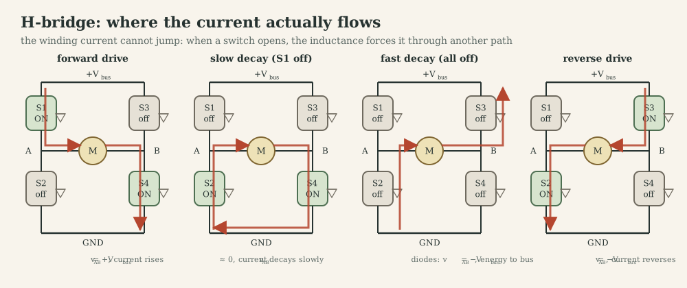
| State | Switches on | Winding voltage $v_{AB}$ | Current (forward) | Mechanical effect |
|---|---|---|---|---|
| Forward drive | S1, S4 | $+V_{\text{bus}}$ | rises | motoring, accelerates forward |
| Slow decay | S2, S4 (or S1, S3) | ≈ 0 | decays as $(v=-e)$ through the low (or high) switches | current keeps producing torque; back-EMF brakes it slowly |
| Fast decay | none (diodes D2, D3) or S2, S3 | $-V_{\text{bus}}$ | decays fast, energy returns to the bus | regenerative braking while current is positive |
| Reverse drive | S2, S3 | $-V_{\text{bus}}$ | builds negative current | motoring in reverse |
| Brake | both low sides on (A4973 BRAKE) | 0 | short-circuited winding: $i=-e/R$ | dynamic braking, motor energy dissipated in $R$ |
| Coast | all off | floats | decays through diodes to zero, then no current | free-wheeling, no torque |
Never turn on S1 and S2 (or S3 and S4) together: that shorts the bus through one leg (shoot-through, J.6).
Bipolar versus unipolar PWM (MF2030 C2). In bipolar (locked anti-phase) PWM, the bridge alternates between forward drive and reverse drive: the average voltage is $(2D-1)V_{\text{bus}}$, the current is never discontinuous, zero speed is $D=0.5$, and the ripple is twice as large. In unipolar (sign-magnitude) PWM, one leg switches while the other is held: drive alternates with slow decay, the average is $D\,V_{\text{bus}}$ in the chosen direction, the ripple is halved and switching losses are lower; the direction is a separate bit.
Four quadrants. Torque (current) and speed each have two signs. Quadrants I and III are motoring ($\tau\omega>0$); II and IV are braking ($\tau\omega<0$), where mechanical energy flows back to the supply. A bench power supply cannot sink current, so regenerated energy charges the bus capacitor. Worked example: stopping the BX4 from its no-load speed (576 rad/s, $J=6.2\cdot10^{-6}$ kg·m², 1.03 J of kinetic energy) into 470 µF at 24 V raises the bus to $\sqrt{24^2+2\cdot1.03/470\,\mu\text{F}}\approx70$ V, above the A4973’s 50 V rating. The A4973 datasheet warns about exactly this in fast-decay mode. A battery absorbs it; a bench supply needs a braking chopper or a clamp.
My MF2043 H-bridge board. The lab-2 board uses an Allegro A4973 full-bridge driver (±1.5 A, 50 V, internal crossover dead time 500 ns, thermal shutdown at 165 °C). Its logic maps directly onto the table above:
| BRAKE | ENABLE | PHASE | MODE | Outputs | Meaning |
|---|---|---|---|---|---|
| H | H | X | H | off | sleep |
| H | H | X | L | off | standby |
| H | L | H | H/L | A high, B low | forward, fast/slow decay during current limiting |
| H | L | L | H/L | A low, B high | reverse, fast/slow decay |
| L | X | X | X | both low | brake |
The internal current limit trips at $I_{\text{trip}}=V_{\text{REF}}/(2R_S)$; after a trip the drivers stay off for $t_{\text{off}}=R_TC_T$, decaying in the mode selected by MODE. The lab drove PHASE with 20 kHz PWM from the mbed controller (locked anti-phase operation) and measured motor current over $R_S$ while a second motor, loaded by a power resistor, acted as a generator. The project page reviews the board’s component values against these formulas.
The MF2103 shield. The STM32 drives two PWM channels (TIM3 CH1 on PB4, CH2 on PA7) and two enable pins (PA5, PA6) of a “DC motor control shield” whose part number is not documented. The firmware sets CCR1 = duty, CCR2 = 0 for one direction and the reverse for the other: sign-magnitude PWM on one leg while the other leg is held low, if the shield’s input logic is the usual “IN = 1 → high side, IN = 0 → low side”. Under that assumption the off-state is slow decay through the two low-side switches, and the average voltage is $D\,V_{\text{bus}}$.
My lab H-bridge. The A4973 board puts the four switches, the current chopper and the logic in one package. Its off-time capacitor, reference divider and supply pins illustrate most of the design choices above; the review is on the project page.
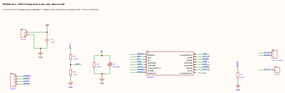
J.5 The three-phase inverter
Three half-bridge legs, six switches, eight states (I.6). Each leg’s output is either $V_{dc}$ or 0; the motor responds only to differences between legs. During dead time each leg’s current flows through a body diode, so the leg voltage depends on the current’s sign rather than on the command (J.6). Current paths for six-step follow I.2; in FOC all three legs switch every period.
A three-phase example. My BLDC torque shield shows a complete inverter:
- three legs of 60 V, 2.8 mΩ MOSFETs (BSC028N06NS);
- a low-side shunt under each leg;
- bulk capacitors plus local decoupling at each leg;
- a TVS on the input;
- a DRV8323S gate driver.
The driver generates its high-side gate voltage with a charge pump (VCP, CPH/CPL on the schematic) instead of bootstrap capacitors, so it avoids the 100 % duty limit discussed in J.6. On the PCB, the power loop (bus capacitor → high side → low side → shunt → ground) is kept short on the left, away from the signal side on the right.
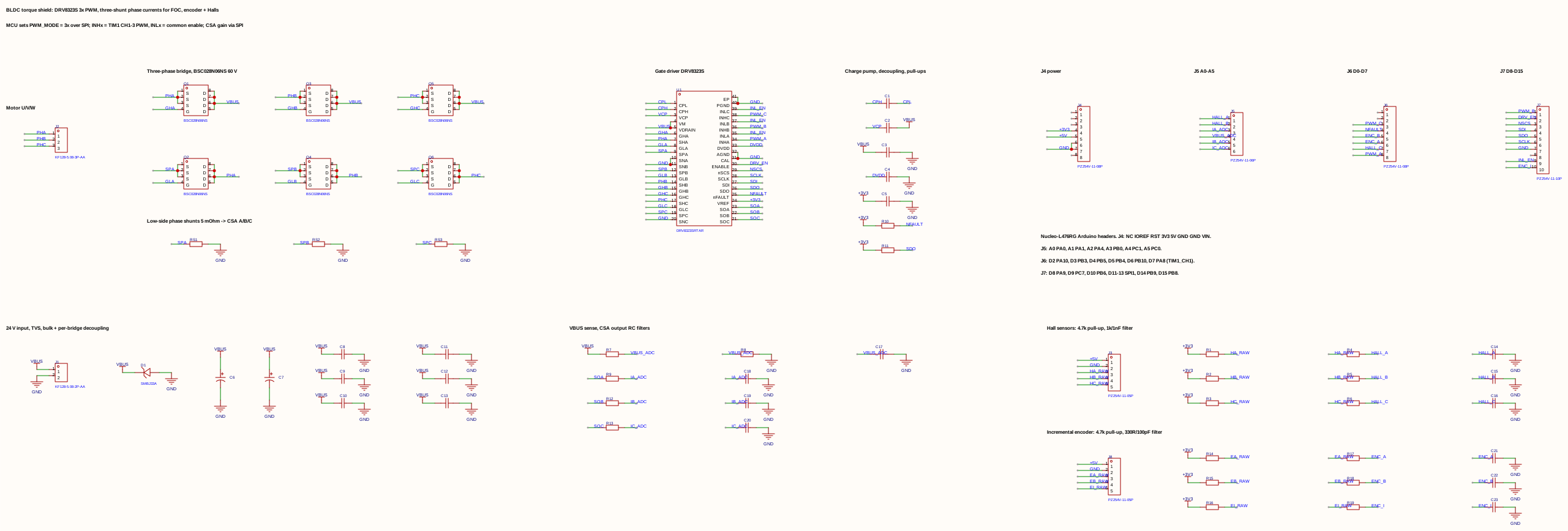
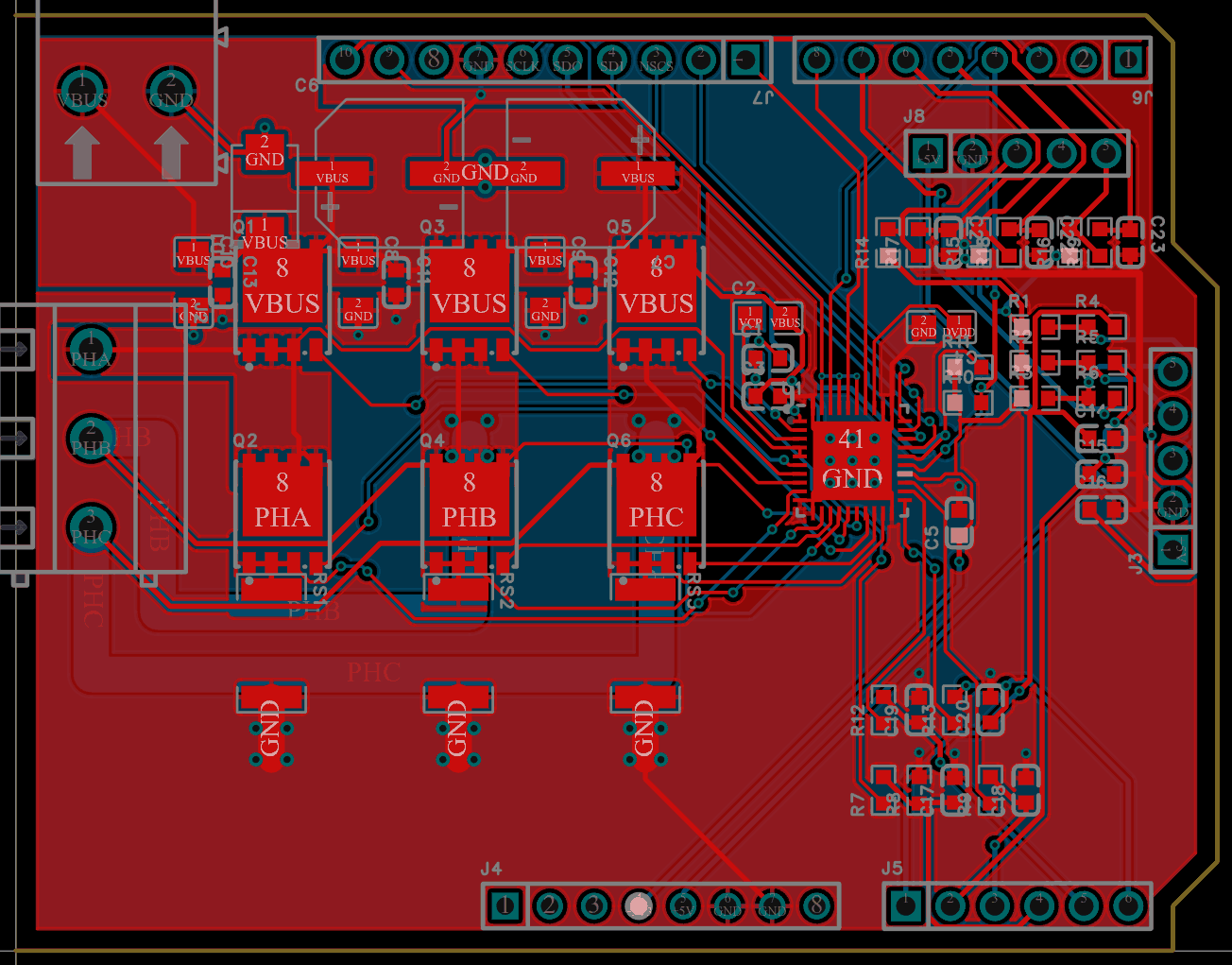
J.6 Gate drivers, bootstrap supplies and dead time
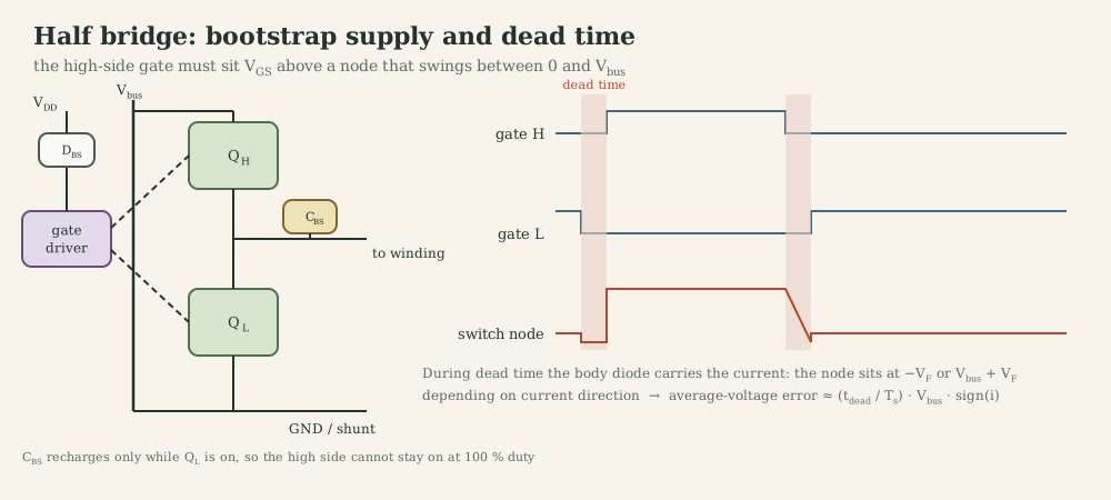
A gate driver translates logic levels into fast gate currents (amps, for nanoseconds), level-shifts the high-side signal, and enforces timing.
Bootstrap. When the low-side switch is on, the switch node is at ground and $C_{BS}$ charges to $V_{DD}$ through $D_{BS}$. When the high side turns on, the switch node rises to $V_{\text{bus}}$ and $C_{BS}$ floats up with it, supplying $V_{GS}$. Consequences: $C_{BS}$ must hold enough charge for the longest on-time (rule of thumb $C_{BS}\ge10\,Q_g/\Delta V$), and 100 % duty is impossible indefinitely because the capacitor is never recharged; drivers impose a maximum duty or need a charge pump.
Shoot-through and dead time. Turn-off is slower than turn-on, so switching one transistor off and the other on at the same instant briefly turns both on: a short circuit across the bus. Dead time $t_d$ (both off) prevents it. During $t_d$ the current freewheels through a body diode, and the switch node sits at $-V_F$ (current flowing out of the leg) or $V_{\text{bus}}+V_F$ (current flowing in) regardless of the command. The result is a voltage error proportional to $t_df_{\text{PWM}}V_{\text{bus}}\,\mathrm{sign}(i)$: 500 ns at 20 kHz on 24 V gives 0.24 V. That is 1 % of the bus, but at low speed and low current it is a large fraction of the needed voltage, it distorts current near zero crossings, and it is the main reason for low-speed torque ripple in FOC. Compensation adds $\pm t_df_{\text{PWM}}V_{\text{bus}}$ to the command according to the measured current sign.
J.7 PWM frequency versus electrical time constant
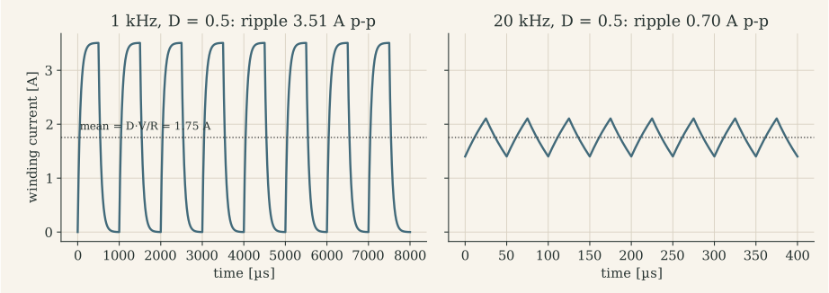
For unipolar PWM in steady state (back-EMF $e\approx DV_{\text{bus}}$, $R$ neglected), the peak-to-peak current ripple is
\[\Delta I\approx\frac{V_{\text{bus}}\,D(1-D)}{L\,f_{\text{PWM}}},\]maximal at $D=0.5$; bipolar PWM doubles it. The ripple produces copper loss ($I_{\text{rms}}^2R$ with no torque), torque ripple, iron loss and acoustic noise, and it biases current measurements that are not sampled at the right instant.
The MF2030 rule of thumb is $10\,T_{\text{PWM}}<\tau_e$. For the BX4 ($\tau_e=76$ µs) that means $f_{\text{PWM}}>130$ kHz; for the coreless Assun motor ($\tau_e=61$ µs), above 160 kHz. Real drives for such motors use 40-100 kHz, accept some ripple, or add series inductance. MF2043 asked the same question with its 2 Ω, 200 µH example: $\tau=0.1$ ms against a 0.5 ms half-period at 1 kHz means the current almost reaches its final value in every half-cycle, and the motor heats without turning. The MF2103 platform runs at 20 kHz (TIM3 ARR = 2000 at 40 MHz), above audibility but with a 0.7 A ripple on a motor rated at 0.48 A continuous. The upper limit on $f_{\text{PWM}}$ comes from switching loss, minimum pulse widths, dead time (which grows as a fraction of the period) and timer resolution.
J.8 Current sensing
| Method | Where | Pros | Cons |
|---|---|---|---|
| Low-side shunt | between bridge and ground | common mode ≈ 0 V, cheap | sees current only when low side conducts; cannot detect shorts to ground |
| High-side shunt | between supply and bridge | sees supply current, detects ground faults | high common mode; needs a high-side amplifier |
| In-line (phase) shunt | in series with the winding | sees real winding current all the time | common mode swings 0 ↔ $V_{\text{bus}}$ at PWM frequency; needs PWM-rejecting amplifier |
| Hall / fluxgate sensor | around the conductor | isolated, no loss | offset drift, bandwidth, cost |
Shunt design. Choose $R_S$ so that full-scale current gives tens to a hundred millivolts (loss $I^2R_S$: 0.23 W for 0.1 Ω at 1.5 A), use a Kelvin (four-wire) connection, and an amplifier whose common-mode range covers the shunt location.
The amplifier side of the sensor (gain, offset, bandwidth, designing backwards from the ADC) is in Part E.4; my lab-4 board’s netlist review is on the project page.
Sampling. Sample at the centre of the PWM pulse (Part F.1) (or of the zero-vector period for low-side shunts in an inverter), where the ripple crosses its average. Trigger the ADC from the PWM timer, not from software (Part M.4). A 12-bit ADC over 3.3 V with a ±1.5 A full-scale sensor resolves 0.73 mA per LSB.
J.9 Voltage sensing and power supply
Measure the bus voltage through a divider into an ADC channel, and use it to scale duty: $D=v^\ast/V_{\text{bus}}$ keeps the loop gain constant as a battery discharges (a nutrunner’s 30 V pack can sag by 20 % under load).
My MF2043 lab-1 supply converts 24 V to 12 V with an LM2576-ADJ buck regulator (52 kHz, trimmer-adjustable feedback) and 12 V to 5 V with an LM317 linear regulator ($V_{\text{out}}=1.25(1+R_2/R_1)=1.25(1+3\,\text{k}/1\,\text{k})=5.0$ V). Two lessons from re-reading the schematic: buck regulators need a fast (Schottky) catch diode, and a standard rectifier such as the 1N4004 on the board adds reverse-recovery loss and noise; and the LM317 needs a minimum load current of about 3.5-10 mA, while a 1 kΩ upper divider resistor draws only 1.25 mA, so at no load the 5 V rail can drift upward (datasheet designs use 120-240 Ω).
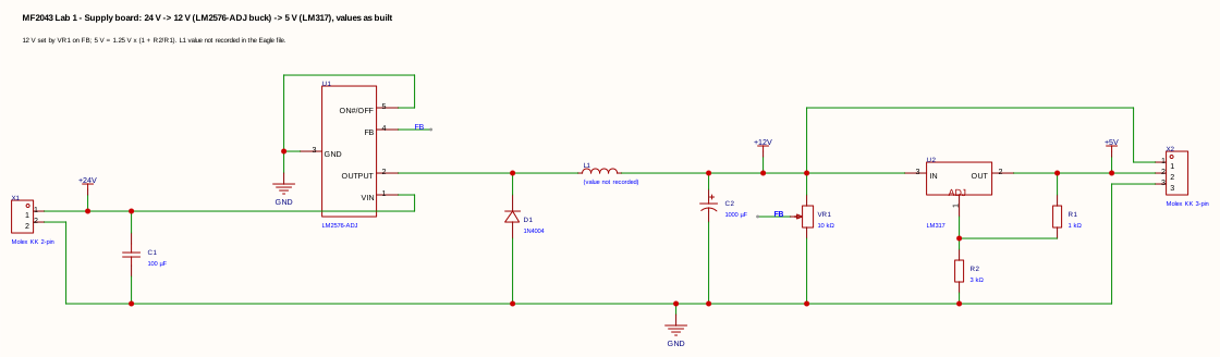
J.10 Protection
| Hazard | Detection | Reaction | Where |
|---|---|---|---|
| Over-current (short, stall) | comparator on shunt, cycle-by-cycle | turn off switches within µs | driver IC (A4973 $I_{\text{trip}}$) or timer break input (STM32 TIM1 BKIN) |
| Sustained overload | $I^2t$ or thermal model in firmware | reduce current limit | firmware, ms to s |
| Over-voltage (regeneration) | bus voltage ADC | brake chopper, stop braking | hardware + firmware |
| Under-voltage | UVLO in gate driver (A4973: 2.75 V on logic supply) | disable outputs | driver IC |
| Over-temperature | die sensor (A4973: 165 °C), NTC on board/motor | shut down, derate | driver IC + firmware |
| Reverse battery | series MOSFET or diode | block | hardware |
| Firmware fault | watchdog, fault handler | safe state (outputs off) | MCU |
The safe state must be chosen per application: all switches off (coast) is safest for the electronics, but a motor that must stop quickly needs braking, and a brake that relies on firmware is not a safety function.
J.11 EMI and EMC
The fast edges that make switching efficient also radiate. The design rules from MF2043 lectures 6-7 and 7.5:
- Minimize hot-loop area: the bus capacitor, high-side and low-side switches form a loop carrying the full switched current; place a ceramic capacitor (100 nF-1 µF) right at the bridge, in addition to bulk capacitance. (My lab-2 board, as drawn, has one 47 µF electrolytic on the 24 V input and no ceramic decoupling at the driver: a first thing to fix.)
- Use a ground plane (the lab-2 prestudy asked for a two-sided board with one side as ground) and separate the power return from the signal ground, joining them at one point near the shunt.
- Control $dv/dt$ with gate resistors: slower edges, less radiation, more switching loss.
- Keep the freewheel/clamp components at the load to keep the high-$di/dt$ loop small (lab 2, question 6).
- Protect inputs with TVS diodes and RC filters against transients (MF2043 lecture 7.5); twist motor leads; filter or shield encoder cables.
What to remember
- Follow the current: every switching state is a different current path.
- Slow decay recirculates current through the bridge; fast decay returns energy to the bus, which can over-charge a bench supply.
- High-side N-MOSFETs need a bootstrap or charge pump; dead time prevents shoot-through and causes a voltage error.
- Choose $f_{\text{PWM}}$ from $\tau_e$: low-inductance motors need high frequencies or tolerate ripple.
- Sample current synchronously with PWM; size gain and offset for the full bidirectional range.
Part K. Embedded foundations: below the abstraction
The controller of Part G is now a few dozen lines of C on an STM32L476 (Cortex-M4F, 40 MHz in MF2103). To trust it, one must know what the processor does with those lines.
K.1 The core: registers, reset and exceptions
Registers. A Cortex-M core has sixteen 32-bit core registers: R0-R12 general purpose, R13 = SP (stack pointer; two banked copies, MSP for handlers and the OS, PSP for threads), R14 = LR (link register: return address of a call, or a special EXC_RETURN value inside a handler), R15 = PC (program counter), plus xPSR (flags, exception number). The M4F adds 32 single-precision floating-point registers.
Reset sequence. The core reads the initial MSP from address 0x0000_0000 and the reset vector from 0x0000_0004 (the vector table, aliased to flash at 0x0800_0000), then runs Reset_Handler, which configures clocks (SystemInit), copies initialized data from flash to RAM (.data), zeroes .bss, and calls main(). Nothing in C is initialized before this code runs.
Exceptions and interrupts. On an interrupt the hardware pushes R0-R3, R12, LR, PC and xPSR onto the current stack (eight words, plus the FPU context if lazy stacking is triggered), loads the handler address from the vector table and runs it in handler mode. The NVIC decides which pending interrupt runs by priority; a higher-priority interrupt preempts a lower one. Entry takes 12 cycles on Cortex-M4 (zero wait-state memory), which at 40 MHz is 0.3 µs: interrupt latency is usually dominated by code that disables interrupts, not by the hardware.
K.2 One address space: memory and peripherals
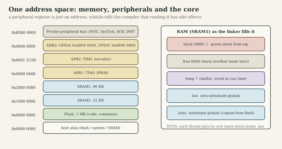
Flash (code, constants), SRAM (variables, stacks), and peripheral registers all have addresses. Writing to 0x4800_0018 does not store a value in memory: it sets pins on GPIO port A. This is memory-mapped I/O, and it is why C pointers are the language of embedded hardware access.
#include <stdint.h>

/* GPIOA base 0x4800 0000, BSRR at offset 0x18 (STM32L4 reference manual) */
#define GPIOA_BSRR (*(volatile uint32_t *)0x48000018U)

GPIOA_BSRR = (1U << 5);          /* set PA5   (bits 0-15 set)   */
GPIOA_BSRR = (1U << (5 + 16));   /* reset PA5 (bits 16-31 reset) */
CMSIS device headers wrap the same addresses in structures (GPIOA->BSRR = GPIO_BSRR_BS5;, exactly the line that enables the bridge in my MF2103 peripherals.c), and the ST HAL wraps those in functions (HAL_GPIO_WritePin). MF2103 used all three levels: raw addresses in tutorial 2, CMSIS in the peripherals module, HAL and CubeMX-generated code for initialization.
K.3 volatile, bit manipulation and read-modify-write
volatile tells the compiler that every read and write of the object is an observable side effect: it must not cache the value in a register, merge accesses, or delete a “useless” loop. Required for peripheral registers and for variables shared with an ISR; not sufficient for thread safety (it gives no atomicity or ordering across cores).
Bit operations:
reg |=  (1U << n);                       /* set bit n            */
reg &= ~(1U << n);                       /* clear bit n          */
reg ^=  (1U << n);                       /* toggle bit n         */
if (reg & (1U << n)) { /* ... */ }       /* test bit n           */
reg = (reg & ~MASK) | ((val << SHIFT) & MASK);   /* write a field */
reg |= x is three operations: load, OR, store. If an interrupt modifies the same register between the load and the store, its change is lost. Hardware offers atomic alternatives: STM32’s BSRR register sets or resets pins without reading; the RP2040 used in 1DT106 gives every register SET/CLR/XOR aliases at fixed address offsets; Cortex-M3/M4 parts may implement bit-banding, where each bit of a region is mirrored as a whole word. Otherwise the read-modify-write must sit inside a critical section (Part L).
Register-level timer set-up for the MF2103 pins. CubeMX generated this in the course; written out, it shows what the generated code does:
/* TIM3: 20 kHz PWM on PB4 (CH1) and PA7 (CH2); timer clock 40 MHz */
RCC->AHB2ENR  |= RCC_AHB2ENR_GPIOAEN | RCC_AHB2ENR_GPIOBEN;
RCC->APB1ENR1 |= RCC_APB1ENR1_TIM3EN;

GPIOB->MODER = (GPIOB->MODER & ~(3U << (4*2))) | (2U << (4*2));     /* PB4 alternate function */
GPIOB->AFR[0] = (GPIOB->AFR[0] & ~(0xFU << (4*4))) | (2U << (4*4)); /* AF2 = TIM3_CH1         */
GPIOA->MODER = (GPIOA->MODER & ~(3U << (7*2))) | (2U << (7*2));     /* PA7 alternate function */
GPIOA->AFR[0] = (GPIOA->AFR[0] & ~(0xFU << (7*4))) | (2U << (7*4)); /* AF2 = TIM3_CH2         */

TIM3->PSC   = 0;                    /* count at 40 MHz                           */
TIM3->ARR   = 2000;                 /* period = 2001 counts -> 19.99 kHz         */
TIM3->CCMR1 = (6U << TIM_CCMR1_OC1M_Pos) | TIM_CCMR1_OC1PE     /* PWM mode 1, preload */
            | (6U << TIM_CCMR1_OC2M_Pos) | TIM_CCMR1_OC2PE;
TIM3->CCER  = TIM_CCER_CC1E | TIM_CCER_CC2E;                     /* enable outputs      */
TIM3->CCR1  = 0; TIM3->CCR2 = 0;
TIM3->CR1   = TIM_CR1_ARPE;         /* buffer ARR too                            */
TIM3->EGR   = TIM_EGR_UG;           /* load the shadow registers                 */
TIM3->CR1  |= TIM_CR1_CEN;          /* start                                     */

/* TIM1: quadrature encoder on PA8 (CH1) and PA9 (CH2), AF1, 16-bit counter */
RCC->APB2ENR |= RCC_APB2ENR_TIM1EN;
/* ... PA8/PA9 to AF1 as above ... */
TIM1->CCMR1 = TIM_CCMR1_CC1S_0 | TIM_CCMR1_CC2S_0;   /* TI1 -> IC1, TI2 -> IC2              */
TIM1->SMCR  = TIM_SMCR_SMS_0 | TIM_SMCR_SMS_1;       /* encoder mode 3: count both edges     */
TIM1->ARR   = 0xFFFF;                                 /* full 16-bit range                    */
TIM1->CR1   = TIM_CR1_CEN;
Three details matter for control. Preload (OCxPE, ARPE) makes a CCR write take effect only at the next update event, so a duty change never produces a glitch mid-period. ARR = 0xFFFF on the encoder timer lets differences of two readings, cast to int16_t, handle counter wrap automatically (K.6). Encoder mode 3 counts every edge of both channels: four counts per encoder line.
K.4 Memory: where data lives and how it fails
The linker places code in .text and constants in .rodata (flash); initialized globals in .data (stored in flash, copied to RAM at reset); zero-initialized globals and statics in .bss; the heap grows upward from the end of .bss; the main stack grows downward from the top of RAM. The 1DT106 examples:
char       rwData[100];         /* .bss   (RAM, zeroed at reset)          */
char       raData[3] = {1, 2, 3};  /* .data  (RAM, initial value in flash) */
const char roData[3] = {1, 2, 3};  /* .rodata (flash only)                 */
The .map file (MF2103’s Keil listings) shows the exact addresses and sizes; arm-none-eabi-objdump -h shows the sections of an ELF.
Static versus dynamic allocation. malloc/free at run time risk running out of memory at an unpredictable moment, leaking, and fragmenting the heap (free memory exists but no single block is large enough), and their execution time is not bounded. Embedded coding standards (MISRA C:2012 Directive 4.12) forbid dynamic allocation after initialization; RTOSes provide fixed-size block pools (Zephyr memory slabs) with deterministic timing instead.
Stack overflow is the classic silent failure: deep call chains, large local arrays, recursion (the 1DT106 recursive factorial with a 100-byte stack) or an ISR running on a thread’s stack overwrite whatever lies below. Detection: canaries (a known pattern at the stack end, checked at context switches; Zephyr CONFIG_STACK_SENTINEL), the MPU (a guard region that faults on access; Zephyr CONFIG_MPU_STACK_GUARD), and measuring the high-water mark (Zephyr thread analyzer, RTX stack watermarking). MF2103 set RTX thread stacks to 1024 bytes; whether that is enough is a measurement, not a guess.
Buffer overflow writes past an array’s end into neighbouring variables; with network input (MF2103 task 3 receives bytes over TCP) every length must be checked.
K.5 Why embedded C differs from desktop C
| Issue | Desktop habit | Embedded reality |
|---|---|---|
| Integer width | int is “big enough” |
int is 32 bits on Cortex-M, 16 on some MCUs: use <stdint.h> (int16_t, uint32_t) |
| Overflow | rare | common: 16-bit counters, fixed-point products; signed overflow is undefined behaviour |
| Mixed signedness | unnoticed | int * uint32_t is computed as unsigned |
| Division | fast | integer division truncates toward zero; dividing before multiplying loses resolution; no hardware divide on Cortex-M0 |
| Floating point | free | single precision in hardware on M4F; double is software-emulated and ~10-50× slower; literal 1.0 is a double, write 1.0f |
| Memory | gigabytes, virtual | kilobytes, no MMU, statically planned |
| Allocation | new, malloc |
static at start-up only |
| Timing | irrelevant | WCET matters (Part M) |
| Optimization | makes code faster | can delete loops and reorder accesses unless volatile/atomics are used |
| I/O | files, streams | registers, ISRs; printf over SWO/UART can take milliseconds |
Fixed point. Without an FPU (or to save ISR time), represent a real number $x$ as an integer $X=\mathrm{round}(x\cdot2^q)$, the Q-format with $q$ fractional bits. Q15 holds values in $[-1,1)$ in an int16_t; a product of two Q15 values is Q30 in an int32_t and is shifted right by 15 to return to Q15. A PI step in Q15 with saturation:
#include <stdint.h>

typedef struct { int16_t kp_q15, ki_q15; int32_t integ_q30; } pi_q15_t;

static inline int16_t sat16(int32_t x)
{
    return (int16_t)(x > INT16_MAX ? INT16_MAX : (x < INT16_MIN ? INT16_MIN : x));
}

int16_t pi_q15_step(pi_q15_t *c, int16_t err_q15)
{
    int32_t p = (int32_t)c->kp_q15 * err_q15;          /* Q30 */
    int32_t i = c->integ_q30 + (int32_t)c->ki_q15 * err_q15;
    int16_t u = sat16((p + i) >> 15);                   /* back to Q15, saturated */
    if (u != (int16_t)((p + i) >> 15)) {                /* saturated: do not integrate */
        return u;
    }
    c->integ_q30 = i;
    return u;
}
(The integrator is limited by conditional integration; a production version also clamps integ_q30 itself so that p + i cannot overflow.) The rules: choose scaling from the physical ranges (current ±1.5 A full scale, speed ±600 rad/s), keep products in a wider type, saturate instead of wrapping, and test against a floating-point reference. MF2007 C6 calls this “scaling of signals”; MF2103’s ±2·10⁹ ↔ ±100 % convention is a fixed-point format with a very large scale factor, chosen to keep resolution, at the price of overflow risk.
C++ in firmware works well with discipline: no exceptions and RTTI (code size, non-deterministic unwinding), no heap after start-up, but constexpr, templates, strong types for units (a Volts type that cannot be added to Amps) and RAII for critical sections (a lock object whose destructor re-enables interrupts) catch errors at compile time.
K.6 Five C pitfalls, found in my own motor-control code
The MF2103 skeleton fixed the interfaces (int16_t Peripheral_Timer_ReadEncoder(void), void Peripheral_PWM_ActuateMotor(int32_t) with ±2·10⁹ meaning ±100 % duty, Controller_PIController(ref, current, millisec)), and my group wrote the bodies. Re-reading them with the topics above gives a compact catalogue of embedded-C pitfalls in control code:
| Pitfall | Line from the code | What goes wrong | Rule |
|---|---|---|---|
| Counter wrap | int16_t rad = encoder - oldencoder; |
nothing: the signed 16-bit difference handles the wrap of the 16-bit timer, as long as fewer than 32 768 counts pass per period | the pattern to keep |
| Division order | -rad * 60 / dt * 1000 / 2048 |
integer division before scaling truncates (exact at 10 ms, lossy at 50 ms) | multiply first: -rad * 60000 / (dt * 2048) |
| Unit slip | draft: (encoder - oldencoder) * 1000 / dt / 60 / 2048 |
divides by 60 instead of multiplying: 3600× too small, zero below 3600 rpm | unit-test every conversion with a known input |
| Mixed signedness | kp*t with int16_t kp, uint32_t t |
computed in unsigned arithmetic; correct only because two’s complement wraps consistently | explicit casts, or float on an FPU |
| Overflow before the clamp | pidout = kp*error + ki*I; and pidout += ...; |
with the rotor held, the sum exceeds 32 bits before it is clamped; signed overflow is undefined and wraps to the opposite sign in practice | compute in int64_t or float, clamp before storing, test the stalled rotor |
The last row is where windup (Part G.11) meets fixed point. The project page replays the submitted code bit-exactly against a motor model: the RTOS version overflows 77 times with the rotor held, and the final version switches to full reverse duty at a 50 ms period. The fixes are standard: int64_t (cheap on a Cortex-M4 via SMULL) or float, an integrator state that is itself clamped, and tests of the saturated cases, not just the nominal step. Part O returns to this as a debugging case.
What to remember
- Registers, vector table and reset handler run before
main; ISRs push eight words and run in handler mode. - Peripherals are addresses;
volatilekeeps every access; read-modify-write is not atomic. - Timer PWM uses preload so duty changes land at the period boundary; encoder differences cast to
int16_thandle wrap. - Plan memory statically; detect stack overflow with canaries or the MPU.
- Watch integer width, signedness and evaluation order; saturate instead of overflowing; test the saturated case.
Part L. Concurrency and synchronization
L.1 Why motor-control firmware is concurrent
A drive does many things at different rates and with different urgency:
| Activity | Rate / trigger | Deadline | Consequence of lateness |
|---|---|---|---|
| PWM generation | 20 kHz | hard, in hardware | none if hardware does it |
| Current sampling + current loop | 10-20 kHz | before next PWM update | wrong voltage applied, current error, instability |
| Speed loop | 1-5 kHz | within its period | degraded damping |
| Position loop, trajectory | 0.1-1 kHz | within its period | tracking error |
| Protection (over-current) | event | microseconds | hardware damage |
| Communication (CAN, UART, TCP) | event | ms to s | stale commands |
| Logging, UI | background | soft | none |
One sequential loop cannot serve all of these: the slowest activity would delay the fastest. Concurrency means structuring the program as several activities that make progress in overlapping time; on a single core they are interleaved by interrupts and a scheduler.
L.2 From super-loop to RTOS
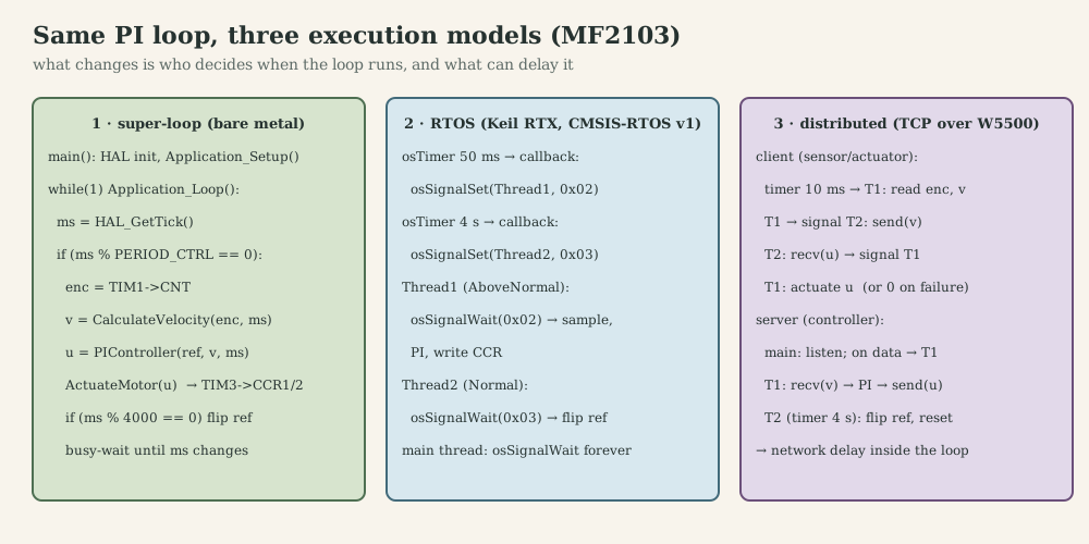
- Super-loop with polling (MF2103 task 1).
while(1)reads the millisecond tick and runs the controller whenms % PERIOD == 0, then busy-waits until the tick changes. Simple and deterministic if everything in the loop is short. Fragile otherwise: if anything in the loop (aprintfover SWO, a slow computation) takes longer than one millisecond at the wrong moment, the equality test misses that tick and the whole control period is skipped. All activities share one timeline. - Foreground/background. The control law runs in a timer interrupt (foreground, precise period); everything else runs in the main loop (background). The standard bare-metal motor-control architecture: the ISR has fixed timing, the background has whatever time is left.
- Cooperative scheduler. Tasks run to completion and return; a dispatcher calls them by period. No preemption means no data races between tasks, but one long task delays all others.
- Preemptive RTOS (MF2103 task 2, Zephyr). Each activity is a thread with a priority; the kernel switches to the highest-priority ready thread whenever an event (interrupt, timer, semaphore) makes it ready. Timing of high-priority work becomes independent of low-priority work, at the cost of context-switch overhead and the need for synchronization.
L.3 Interrupt service routines
An ISR runs when hardware asks: ADC conversion complete, timer update, encoder index, UART byte, over-current. Rules:
- Keep it short and bounded. Its execution time adds to the latency of every lower-priority interrupt and thread.
- Never block: no mutex locks, no waiting on semaphores, no
printf, nomalloc. - Clear the interrupt flag, or the ISR re-enters immediately.
- Share data deliberately: variables written in an ISR and read elsewhere are
volatile, and multi-word data needs a consistent-read protocol (L.5).
Deferred interrupt processing moves the work out of the ISR into a thread. The 1DT106 Zephyr example does exactly this with a button:
K_SEM_DEFINE(sem, 0, 1);                         /* initial count 0, limit 1 */

void button_isr(const struct device *dev, struct gpio_callback *cb, uint32_t pins)
{
    k_sem_give(&sem);                            /* signal only; no work here */
}

void button_task(void *a, void *b, void *c)
{
    for (;;) {
        k_sem_take(&sem, K_FOREVER);             /* sleep until the ISR signals */
        gpio_pin_toggle_dt(&led);                /* the actual handling         */
    }
}
K_THREAD_DEFINE(button_tid, 500, button_task, NULL, NULL, NULL, 5, 0, 0);
The motor-control version of the same pattern: ADC end-of-conversion ISR → semaphore → control thread computes the new duty → writes the timer’s CCR register. For a 10 kHz current loop, the thread wake-up overhead (several microseconds) is a significant fraction of the 100 µs period, so the current loop itself usually stays in the ISR and only slower loops are deferred (Part N.5).
L.4 Threads, priorities and context switches
A thread has an entry function, its own stack, a priority, and a state: running (on the CPU), ready (could run, waiting for the CPU) or blocked (waiting for time, a semaphore, a message). The kernel keeps a ready list and always runs the highest-priority ready thread (preemptive priority scheduling); equal priorities may time-slice (round-robin, disabled in MF2103 RTX).
Context switch on Cortex-M. The kernel pends the low-priority PendSV exception; its handler saves R4-R11 (and FPU registers if used) of the outgoing thread on that thread’s stack (the hardware already stacked R0-R3, R12, LR, PC, xPSR), stores the stack pointer (PSP) in the thread’s control block, loads the next thread’s PSP and restores its registers. A few hundred cycles: microseconds at 40 MHz. Deferring the switch to PendSV, which has the lowest priority, means switches never happen in the middle of a higher-priority ISR.
L.5 Shared resources and synchronization, with motor-control examples
Race condition. Two activities access shared data, at least one writes, and the result depends on timing. In a drive:
- The speed thread writes the current reference
i_ref(float, one 32-bit store: atomic on Cortex-M) while the current ISR reads it: harmless. But if the reference is a structure{i_d_ref, i_q_ref}written field by field, the ISR can read one old and one new value: a torn read that can produce a short torque spike. - The ISR updates a 64-bit position counter
pos += delta; a thread reading it with two 32-bit loads can see the high word from before and the low word from after a carry. - A communication thread changes
kpandkiwhile the controller runs: the controller may use the newkpwith the oldkifor one step, and if it readskitwice, two different values in one step.
Tools, from lightest to heaviest:
| Mechanism | What it guarantees | Usable from ISR | Typical motor-control use | Failure if misused |
|---|---|---|---|---|
Atomic variable (atomic_t, C11 _Atomic, LDREX/STREX) |
one indivisible read-modify-write | yes | fault flags, counters, a single reference value | multi-word data still tears |
Critical section (disable IRQs / irq_lock()) |
nothing else runs | yes | copying a multi-word state snapshot | if long: interrupt latency and jitter for everyone |
| Double buffer + sequence counter | consistent multi-word snapshot, writer never blocks | writer yes | ISR publishes {i_a, i_b, θ, t}; threads read a coherent set |
reader must retry |
| Mutex | mutual exclusion with ownership, priority inheritance | no | shared SPI bus between encoder/IMU and Ethernet chip; shared parameter set | deadlock, priority inversion without inheritance, cannot use in ISR |
| Binary semaphore | signalling (count 0/1) | give: yes | ADC ISR wakes control thread | lost wake-ups if the thread is late (count saturates at 1) |
| Counting semaphore | counts events or free resources | give: yes | number of filled sample buffers; encoder index pulses | count drift if give/take unbalanced |
| Message queue | copies data between producer and consumer, buffers bursts | put: yes (no wait) | setpoints from comms to motion thread; log records to logger | full queue: block (bad in control) or drop (decide which) |
| Event flags / thread signals | several boolean events, wait for any/all | set: yes | tightening state machine: TORQUE_REACHED, ANGLE_LIMIT, FAULT |
flags are not counters: repeated events merge |
What can fail in the ADC → semaphore → thread → PWM chain:
- The thread is not the highest-priority ready thread when the semaphore is given: it runs late, the new CCR value misses the next update event, and the voltage is applied one PWM period later than designed (extra delay, Part M).
- Two conversions complete before the thread runs: the binary semaphore saturates at 1, one sample is silently skipped.
- The ADC data register is overwritten by the next conversion before the thread reads it: use DMA into a buffer, or copy the result inside the ISR.
- The thread writes CCR while the timer is between its compare and update events with preload disabled: a glitch pulse.
- Someone adds a
printfin the thread: milliseconds of delay at exactly the wrong time.
L.6 Classic failure modes
Priority inversion. A low-priority thread L holds a mutex; high-priority H blocks on it; medium-priority M (which does not need the mutex) preempts L, so H waits for M: H’s effective priority has dropped below M’s. MF2103’s exam answer key is careful about the definition: H simply waiting for L while L holds the lock is ordinary blocking; it is inversion only when an unrelated medium-priority thread prolongs it. Priority inheritance (L temporarily runs at H’s priority while holding the mutex) bounds it; Zephyr’s k_mutex and CMSIS-RTOS2 mutexes (with osMutexPrioInherit) implement it. Semaphores have no owner and therefore no inheritance, which is one reason to use a mutex, not a binary semaphore, for mutual exclusion.
Deadlock (deadly embrace). Thread 1 locks A then B; thread 2 locks B then A. If each gets its first lock, both wait forever. Prevention: a global lock order, or never holding two locks at once, or timeouts with recovery.
Lost wake-up. A thread checks a condition, decides to wait, but the event arrives between the check and the wait. Kernel primitives that latch the event (semaphores, flags) avoid it; ad-hoc boolean flags plus sleep do not.
Non-reentrant functions. A function using static or global state (the 1DT106 display() example with a global error flag, strtok, many printf implementations) breaks when called from two threads or from a thread and an ISR.
Starvation. A high-priority thread that never blocks starves everything below it. Every periodic thread must block between periods.
L.7 Case study: synchronization in my MF2103 RTOS code
In the RTOS version, two RTX virtual timers fire every 50 ms and 4 s; their callbacks call osSignalSet() to wake the control thread (above-normal priority) and the reference thread (normal). This is correct deferred processing: the callbacks only signal. Shared globals (reference, velocity, control) are single int32_t values written by one thread each: individually atomic on Cortex-M, so no tearing.
The distributed server has a real race: its reference thread calls Controller_Reset(), which clears the integrator and pidout, while the communication thread may be in the middle of Controller_PIController() using them. Whether it bites depends on priorities (the reference thread is above normal and can preempt the PI computation between two statements). The fix is to make the reset a request (an atomic flag) that the control thread applies at the start of its next step, so only one thread ever touches controller state. The client runs its two threads in lockstep with signals (sample → send/receive → actuate), which serializes them; its weakness is timing, not data (Part M.6).
What to remember
- Drives are concurrent because rates and deadlines differ by orders of magnitude.
- Super-loop → foreground/background ISR → cooperative → preemptive RTOS; each step buys timing isolation and costs synchronization.
- ISRs: short, non-blocking, signal threads; deferred processing via semaphores.
- Pick the lightest primitive that is correct: atomics, then double buffers, then mutexes; semaphores signal, mutexes protect, queues transfer.
- Priority inversion needs a third (medium) thread; priority inheritance bounds it; lock ordering prevents deadlock.
Part M. Real-time systems and control timing
M.1 Fast is not the same as real-time
Fast software has a small average execution time. Real-time software produces correct results at the right time: the value of a result depends on when it arrives. A current controller that computes the perfect duty cycle 20 µs after the PWM update has taken effect has applied the wrong voltage for a whole period, however fast it was on average.
| Term | Meaning | Drive example |
|---|---|---|
| Deadline | latest acceptable completion time | new CCR before the next PWM update event |
| Hard real-time | a missed deadline is a failure | over-current shutdown, current loop |
| Firm | a late result is useless but not dangerous | a speed sample that arrives after the next one |
| Soft | lateness degrades quality | logging, UI, telemetry |
| Release time | when a job becomes ready | timer tick, ADC end of conversion |
| Latency | delay from event to response start (or to output) | ADC trigger → ISR entry; sample → actuation |
| Jitter | variation of latency or period from one job to the next | ±5 µs of current-loop start time |
| WCET | worst-case execution time | longest path through the FOC ISR, with all branches and cache misses |
| Response time | release to completion, including preemption | speed thread incl. current ISR interference |
M.2 Where timing variation comes from
- Interrupt latency: hardware entry is fixed (12 cycles on Cortex-M4), but any code that disables interrupts (critical sections, kernel locks,
__disable_irq) delays entry by its own length. - Preemption by higher-priority interrupts and threads.
- Variable execution paths: saturation branches, sector-dependent SVPWM code, division, software floating point.
- Memory effects: flash wait states and prefetch/cache hit or miss; DMA competing for the bus.
- Kernel overhead: tick handling, timer lists, context switches.
- Communication: SPI or network transfers inside the loop.
M.3 Schedulability
Rate-monotonic scheduling (RMS) assigns fixed priorities by period (shorter period, higher priority). For $n$ independent periodic tasks with deadlines equal to periods, a sufficient condition is
\[U=\sum_{i=1}^{n}\frac{C_i}{T_i}\le n\big(2^{1/n}-1\big),\]which tends to $\ln2\approx0.69$. Earliest-deadline-first (EDF) schedules by absolute deadline and is optimal up to $U\le1$, at the cost of dynamic priorities. MF2103 exam (VT2019): three threads with \(\{C,T\}=\{0.5,5\},\{3.5,10\},\{4,20\}\) (worst-case $C$) give $U=0.10+0.35+0.20=0.65$; adding an aperiodic thread with $C=1$ under the 4-task bound $U(4)\approx0.76$ requires $1/T_4\le0.11$, so a minimum inter-arrival time of about 10.
The utilization test is only sufficient. Response-time analysis is exact for fixed priorities: the worst-case response time of task $i$ solves
\[R_i=C_i+\sum_{j\in hp(i)}\Big\lceil\frac{R_i}{T_j}\Big\rceil C_j ,\]by fixed-point iteration starting at $R_i=C_i$. A drive task set (illustrative WCETs for a Cortex-M4):
| Task | $C$ | $T$ | Priority | $R$ (computed) | Deadline met? |
|---|---|---|---|---|---|
| Current-loop ISR | 25 µs | 100 µs | 1 (highest) | 25 µs | yes |
| Speed thread | 60 µs | 1 ms | 2 | 85 µs | yes |
| Position / trajectory | 200 µs | 10 ms | 3 | 360 µs | yes |
| Communication | 1 ms | 20 ms | 4 | 1.77 ms | yes |
| Logging | 2 ms | 100 ms | 5 | 4.68 ms | yes |
Total utilization 0.40, well under the 5-task bound of 0.74. The numbers make the architecture visible: the current ISR takes a quarter of the CPU, so its WCET dominates everything else; doubling it would push the speed thread’s response time and jitter up accordingly.
M.4 Control meets timing: delay and jitter
A constant delay $T_d$ between sampling and actuation is a factor $e^{-sT_d}$ in the loop: it subtracts phase $\omega T_d$ at every frequency. At a 1 kHz current-loop crossover, 50 µs of delay costs 18°, 80 µs costs 29°, and a full 100 µs sample of delay costs 36°, a large part of a typical 45-60° phase margin. A constant delay can be designed for (include $z^{-1}$ in the discrete plant, advance the Park angle by $1.5\,\omega_eT_s$). Jitter cannot be compensated in the same way, because each sample sees a different delay and a different sampling interval.
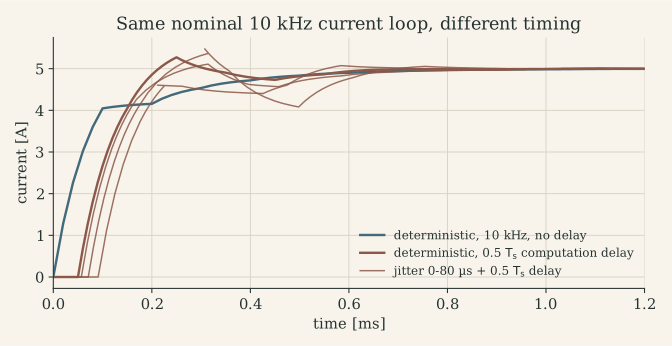
This answers the question “is a nominal 10 kHz controller with large jitter the same as a deterministic 10 kHz controller?”: no. The jittered loop is a time-varying system whose worst case is worse than any single delay value suggests; analysis tools such as Jitterbug compute the cost, but the engineering answer is to remove the jitter at its source by triggering sampling and actuation from hardware.
M.5 Synchronizing everything to the PWM timer
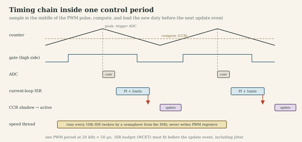
The deterministic chain on an STM32 with an advanced timer (TIM1):
- TIM1 counts up and down (centre-aligned PWM, 20 kHz) and generates complementary outputs with hardware dead time.
- At the counter peak (middle of the high-side pulse in this drawing; the zero-vector centre for low-side shunts), TIM1’s trigger output starts an ADC injected conversion of the phase currents: no software in the sampling path, zero jitter.
- The ADC end-of-conversion interrupt runs the current loop.
- The ISR writes the new duty into the CCR shadow registers; the timer transfers them at the next update event (the counter valley), so the new voltage starts at a known time.
- A repetition counter or a software counter in the ISR wakes the speed thread every tenth period.
The control delay is now a fixed fraction of the period (sampling at the peak, update at the next valley: half a period, or 1.5 periods if the ISR finishes after that valley) and can be modelled exactly. The design constraint becomes WCET of the ISR < time from conversion end to the update event.
Sampling frequency, task period and plant dynamics are tied together:
| Quantity | Chosen from | Example (BX4 drive) |
|---|---|---|
| PWM frequency | $\tau_e$, switching loss, audibility | 20 kHz |
| Current-loop rate | = PWM rate or a submultiple | 10-20 kHz |
| Current-loop bandwidth | ≤ 1/10 of loop rate, phase margin with delay | 1 kHz |
| Speed-loop rate and bandwidth | 5-10× below current loop | 1 kHz, ~100 Hz |
| Position loop | 5-10× below speed loop | 100 Hz-1 kHz |
| Mechanical time constant | plant | $\tau_m=4.6$ ms |
| Encoder speed resolution | counts per revolution × period | sets the useful speed-loop rate |
M.6 Case study: timing in my MF2103 firmware generations
Super-loop. The period is set by polling ms % PERIOD_CTRL == 0 on a 1 ms tick: the sampling instant has up to 1 ms of uncertainty relative to the true tick edge, and any body longer than 1 ms at the boundary skips a whole period. With a 50 ms period and a motor time constant of 8 ms, the motor settles inside every period, so the closed loop is quasi-static and tolerant; with a 10 ms period the same jitter is ten times more significant relative to the period.
RTOS. Virtual timers signal the control thread; the period is now kernel-timed, and the RTX Event Viewer showed the expected ordering of the control and reference threads. Remaining jitter comes from the timer thread’s priority relative to the control thread and from ISRs.
Distributed control over TCP. The client samples the encoder, sends the speed over TCP (W5500 over SPI), waits for the server to compute and return the control value, then actuates. Every control period now contains SPI transfers, two network traversals, the server’s scheduling and a blocking recv(): the sample-to-actuation latency and its jitter depend on the network. Two good choices in the code: Nagle’s algorithm was disabled (SF_TCP_NODELAY), and on any send or receive failure the client sets the duty to zero (fail-safe). Two weaknesses: recv() blocks without a timeout, so a slow server stalls the client’s control thread, and TCP’s retransmission on loss can add hundreds of milliseconds. Real-time networked control uses deterministic buses (CAN, EtherCAT, TSN) or at least UDP with deadlines and stale-data rules, and the controller usually sits next to the actuator. The distributed systems note covers CAN, FlexRay and TSN.
How to measure timing: toggle a GPIO at ISR entry and exit and capture it with a logic analyzer or oscilloscope (period, jitter and execution time in one trace); use the cycle counter (DWT CYCCNT on Cortex-M4) for WCET measurements; use the RTOS trace (RTX Event Viewer, Zephyr tracing / SEGGER SystemView) for thread interactions.
What to remember
- Real-time = correct value at the correct time; specify deadlines, latency, jitter and WCET.
- RMS bound $n(2^{1/n}-1)$ is sufficient; response-time analysis is exact for fixed priorities.
- Delay costs phase $\omega T_d$; constant delay can be designed for, jitter must be removed.
- Trigger the ADC from the PWM timer, compute in the end-of-conversion ISR, update through preload registers.
- Never put a network round trip inside a fast control loop.
Part N. RTOS in practice: CMSIS-RTOS and Zephyr
N.1 What I used: Keil RTX through CMSIS-RTOS v1 (MF2103)
The MF2103 task-2 set-up exposes the practical details any RTOS port involves:
- Configuration (
RTX_Conf_CM.c): default and main thread stacks 1024 bytes, kernel timer clock 40 MHz (equal to the core clock), round-robin off (pure priority scheduling). - Who owns SysTick? The ST HAL uses SysTick for
HAL_GetTick(); RTX uses it for the kernel tick. Both defineSysTick_Handler,SVC_HandlerandPendSV_Handler, so the build fails until CubeMX is told not to generate them and their NVIC priorities are set to SVC 14, PendSV 15 and SysTick 15 (lowest).SysTick_ms()was then re-implemented asreturn os_time;. - Error trapping: a breakpoint in
os_error()catches stack overflows and object-creation failures. - API used:
osThreadDef/osThreadCreate,osTimerDef/osTimerCreate/osTimerStart(virtual timers whose callbacks run in the RTX timer thread),osSignalSet/osSignalWait(per-thread event flags; CMSIS-RTOS2 calls them thread flags),osKernelInitialize/osKernelStart.
N.2 Zephyr: project structure and build
Zephyr is an open-source RTOS with a kernel, a device-driver model, networking, and a build system based on CMake, Kconfig and devicetree. The 1DT106 course used it on the Raspberry Pi Pico (RP2040); the MF2103 board, the Nucleo-L476RG, is also an officially supported Zephyr board (nucleo_l476rg), and so is the W5500 Ethernet shield used in MF2103 (wiznet_w5500).
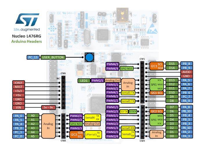
motor_app/
├── CMakeLists.txt          # find_package(Zephyr) + target_sources(app ...)
├── prj.conf                # Kconfig options: what to build into the image
├── boards/
│   └── nucleo_l476rg.overlay   # devicetree changes for this board
└── src/
    └── main.c
west build -b nucleo_l476rg motor_app            # configure and build
west build -b nucleo_l476rg motor_app -- -DSHIELD=wiznet_w5500   # with the Ethernet shield
west flash                                        # program through the ST-LINK
west debug                                        # GDB session via OpenOCD/pyOCD
Board = architecture + SoC + board. Zephyr reuses arch/arm (Cortex-M), the SoC layer (STM32L4) and adds a board file (pins, clocks, on-board LEDs and buttons). An application changes the board only through an overlay.
N.3 Devicetree and Kconfig
Devicetree describes hardware: which peripherals exist, at which addresses, with which pins and properties. Board files define the SoC; overlays enable and configure nodes for the application; bindings (YAML) define which properties a node of a given compatible accepts. At build time the tree is compiled into C macros, so drivers and applications refer to hardware by node, not by address. The 1DT106 example defines an LED and a button and gives them aliases:
/ {
    aliases { led = &led0; btn = &button0; };
    leds    { compatible = "gpio-leds";
              led0: led_0 { gpios = <&gpio0 0 GPIO_ACTIVE_HIGH>; }; };
    buttons { compatible = "gpio-keys";
              button0: button_0 { gpios = <&gpio0 20 GPIO_ACTIVE_HIGH>; }; };
};
and the C code obtains them with GPIO_DT_SPEC_GET(DT_ALIAS(led), gpios).
Kconfig selects software: CONFIG_GPIO=y builds the GPIO driver, CONFIG_LOG=y the logging subsystem. Options live in prj.conf; west build -t menuconfig explores them interactively.
N.4 Generic RTOS concepts and their Zephyr APIs
| Concept | Zephyr API | Notes for a drive |
|---|---|---|
| Thread | K_THREAD_DEFINE, k_thread_create |
own stack; priority below 0 is cooperative (not preempted by other threads), 0 and above preemptible; lower number = higher priority |
| Sleep / periodic wait | k_msleep, k_sleep, k_timer_status_sync |
use a k_timer for drift-free periods |
| Timer | K_TIMER_DEFINE, k_timer_start |
the expiry function runs in ISR context |
| Deferred work | k_work, work queues |
run short jobs in a thread context, e.g. after an ISR |
| Semaphore | K_SEM_DEFINE, k_sem_give, k_sem_take |
give allowed from ISRs |
| Mutex | K_MUTEX_DEFINE, k_mutex_lock |
owner, recursive, priority inheritance; not from ISRs |
| Message queue | K_MSGQ_DEFINE, k_msgq_put, k_msgq_get |
fixed-size items copied; K_NO_WAIT from ISRs |
| Events | k_event_post, k_event_wait |
wait for any/all of 32 bits |
| Polling several objects | k_poll |
one thread waits on semaphores, queues and signals together |
| Atomics | atomic_t, atomic_set, atomic_get, atomic_cas |
lock-free flags and indices |
| Critical section | irq_lock, irq_unlock |
keep to a few microseconds |
| Interrupts | IRQ_CONNECT, IRQ_DIRECT_CONNECT, zero-latency flag |
zero-latency IRQs must not call kernel APIs |
| Memory | K_HEAP_DEFINE, k_mem_slab, CONFIG_STACK_SENTINEL, CONFIG_MPU_STACK_GUARD |
prefer slabs (fixed blocks); libc malloc discouraged |
| Logging | LOG_MODULE_REGISTER, LOG_INF, CONFIG_LOG_MODE_DEFERRED |
deferred mode formats messages in a low-priority thread |
| Diagnostics | CONFIG_THREAD_ANALYZER, CONFIG_ASSERT, k_sys_fatal_error_handler |
stack high-water marks, assertions, fault reporting |
N.5 Device drivers for motor control, and their limits
Zephyr’s generic APIs cover a brushed-DC drive like MF2103’s: PWM (pwm_set_dt(&spec, period_ns, pulse_ns)), GPIO, ADC (adc_read, with sequences and asynchronous completion), and the STM32 quadrature decoder (st,stm32-qdec, read through the sensor API as a rotation angle). They do not cover what a three-phase inverter needs: complementary outputs with dead time, centre-aligned counting, break inputs, and ADC conversions triggered by a timer event at a precise point in the PWM period. For those, a Zephyr application configures the timer and ADC through the vendor’s low-level headers (ST’s stm32_ll_tim.h and stm32_ll_adc.h, shipped in Zephyr’s hal_stm32 module), disables the corresponding generic driver node in devicetree so two drivers do not fight over one peripheral, and connects its own interrupt handler.
N.6 Design 1: the MF2103 speed controller ported to Zephyr
Keeping the MF2103 wiring, a sketch (not compiled here; check pinctrl node names against stm32l476rgtx-pinctrl.dtsi of your Zephyr version):
/* boards/nucleo_l476rg.overlay */
&timers3 {
    status = "okay";
    st,prescaler = <0>;
    pwm3: pwm {
        status = "okay";
        pinctrl-0 = <&tim3_ch1_pb4 &tim3_ch2_pa7>;
        pinctrl-names = "default";
    };
};

&timers1 {
    status = "okay";
    qdec1: qdec {
        compatible = "st,stm32-qdec";
        status = "okay";
        pinctrl-0 = <&tim1_ch1_pa8 &tim1_ch2_pa9>;
        pinctrl-names = "default";
        st,counts-per-revolution = <2048>;   /* assumed, as in the MF2103 firmware */
    };
};

/ {
    zephyr,user {
        pwms = <&pwm3 1 50000 0>, <&pwm3 2 50000 0>;          /* 50 us period = 20 kHz */
        enable-gpios = <&gpioa 5 GPIO_ACTIVE_HIGH>, <&gpioa 6 GPIO_ACTIVE_HIGH>;
    };
};
#include <zephyr/kernel.h>
#include <zephyr/drivers/pwm.h>
#include <zephyr/drivers/gpio.h>
#include <zephyr/sys/atomic.h>
#include <stm32_ll_tim.h>
#include <math.h>

#define KP  4.0e-4f     /* duty per rpm   (tune on the rig) */
#define KI  4.0e-2f     /* duty per rpm·s (tune on the rig) */
#define KAW 1.0e2f      /* anti-windup gain, about 1/Ts     */

#define USER DT_PATH(zephyr_user)
static const struct pwm_dt_spec pwm_cw  = PWM_DT_SPEC_GET_BY_IDX(USER, 0);
static const struct pwm_dt_spec pwm_ccw = PWM_DT_SPEC_GET_BY_IDX(USER, 1);
static const struct gpio_dt_spec en_a = GPIO_DT_SPEC_GET_BY_IDX(USER, enable_gpios, 0);
static const struct gpio_dt_spec en_b = GPIO_DT_SPEC_GET_BY_IDX(USER, enable_gpios, 1);

static atomic_t reference_rpm = ATOMIC_INIT(2000);   /* written by the reference/comms thread */
K_TIMER_DEFINE(ctrl_timer, NULL, NULL);

static void actuate(float duty)                      /* duty in [-1, 1] */
{
    uint32_t pulse = (uint32_t)(fabsf(duty) * pwm_cw.period);
    pwm_set_pulse_dt(duty >= 0.0f ? &pwm_cw  : &pwm_ccw, pulse);
    pwm_set_pulse_dt(duty >= 0.0f ? &pwm_ccw : &pwm_cw,  0);
}

static void control_thread(void *a, void *b, void *c)
{
    const float Ts = 0.010f;                         /* 10 ms                          */
    int16_t last = (int16_t)LL_TIM_GetCounter(TIM1);
    float integ = 0.0f;

    gpio_pin_configure_dt(&en_a, GPIO_OUTPUT_ACTIVE);
    gpio_pin_configure_dt(&en_b, GPIO_OUTPUT_ACTIVE);
    k_timer_start(&ctrl_timer, K_MSEC(10), K_MSEC(10));

    for (;;) {
        k_timer_status_sync(&ctrl_timer);            /* drift-free period              */
        int16_t now = (int16_t)LL_TIM_GetCounter(TIM1);
        float rpm = -(float)(int16_t)(now - last) * 60.0f / (2048.0f * Ts);
        last = now;

        float e = (float)atomic_get(&reference_rpm) - rpm;
        float u = KP * e + integ;
        float u_sat = fminf(fmaxf(u, -1.0f), 1.0f);
        integ += KI * Ts * e + KAW * (u_sat - u);    /* back-calculation anti-windup   */
        actuate(u_sat);
    }
}
K_THREAD_DEFINE(ctrl_tid, 1024, control_thread, NULL, NULL, NULL, 2, 0, 0);
The structure answers the MF2103 problems directly: the period comes from a kernel timer rather than from polling, the controller state belongs to one thread (no reset race), the reference crosses threads through an atomic, floating point on the M4F’s FPU replaces the overflow-prone integer arithmetic, and the network (Zephyr’s BSD sockets over the W5500 shield) lives in a lower-priority thread that exchanges data through a message queue and never blocks the loop.
N.7 Design 2: a PWM-synchronous drive architecture
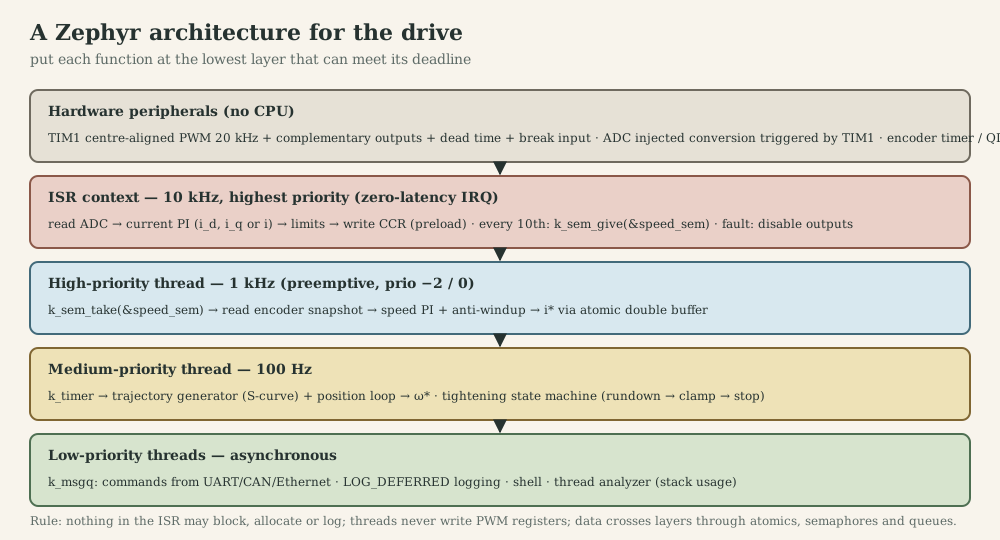
For the BLDC or PMSM version of the drive, with the rates PWM 20 kHz, current loop 10 kHz, speed loop 1 kHz, position loop 100 Hz:
| Function | Layer | Why there |
|---|---|---|
| PWM generation, dead time, complementary outputs, over-current break | timer hardware (TIM1) | must be exact to nanoseconds and survive a software crash |
| Current sampling instant | ADC triggered by TIM1 | zero jitter, synchronized to the PWM centre |
| Current loop (FOC or DC current PI), 10 kHz | direct ISR on ADC end-of-conversion, highest priority | deadline is the next PWM update (< 100 µs); thread wake-up would cost too much |
| Speed loop, 1 kHz | cooperative or high-priority thread woken every 10th ISR | needs floating point and a few tens of µs; tolerates µs jitter |
| Position loop and trajectory, 100 Hz | medium-priority thread on a k_timer |
slower, longer computations (S-curves, state machine) |
| Tightening state machine | same thread or its own | sequencing, limits, fault handling |
| Communication (CAN, UART, Ethernet) | low-priority thread, k_msgq to the position thread |
asynchronous, may block on I/O |
| Logging, shell, diagnostics | lowest priority, deferred logging | never in the control path |
The interrupt handler and the hand-over to the speed thread:
#include <zephyr/kernel.h>
#include <zephyr/irq.h>
#include <zephyr/sys/atomic.h>
#include <stm32_ll_adc.h>
#include <stm32_ll_tim.h>

struct iref { float iq; float id; };
static struct iref ref_buf[2];              /* written by the speed thread           */
static atomic_t ref_active;                 /* index the ISR reads                   */
K_SEM_DEFINE(speed_sem, 0, 1);

ISR_DIRECT_DECLARE(adc_isr)
{
    static uint32_t div;
    LL_ADC_ClearFlag_JEOS(ADC1);
    float ia = adc_to_amps(LL_ADC_INJ_ReadConversionData12(ADC1, LL_ADC_INJ_RANK_1));
    float ib = adc_to_amps(LL_ADC_INJ_ReadConversionData12(ADC1, LL_ADC_INJ_RANK_2));
    const struct iref *r = &ref_buf[atomic_get(&ref_active)];

    foc_step(ia, ib, encoder_angle(), r->id, r->iq);   /* Clarke, Park, PIs, SVPWM -> CCRx */

    if (++div == 10) { div = 0; k_sem_give(&speed_sem); }
    ISR_DIRECT_PM();
    return 1;                                /* ask the kernel to check for a reschedule */
}

static void speed_thread(void *a, void *b, void *c)
{
    for (;;) {
        k_sem_take(&speed_sem, K_FOREVER);
        float iq = speed_pi_step(speed_reference(), speed_estimate());
        int next = 1 - (int)atomic_get(&ref_active);
        ref_buf[next] = (struct iref){ .iq = iq, .id = 0.0f };
        atomic_set(&ref_active, next);       /* publish: the ISR sees old or new, never a mix */
    }
}
K_THREAD_DEFINE(speed_tid, 1536, speed_thread, NULL, NULL, NULL, -1, 0, 0);

void drive_init(void)
{
    /* TIM1: centre-aligned 20 kHz, complementary outputs, dead time, TRGO -> ADC injected (LL calls) */
    IRQ_DIRECT_CONNECT(ADC1_2_IRQn, 0, adc_isr, 0);
    irq_enable(ADC1_2_IRQn);
}
Design decisions and their reasons:
- Direct ISR, not zero-latency. A zero-latency interrupt is never delayed by the kernel’s own critical sections, but it may not call kernel APIs, so it could not give the semaphore. If kernel-induced jitter proves too large, make the current ISR zero-latency and pace the speed thread from a second, ordinary interrupt (for example the timer’s repetition-counter update every tenth period).
- Double buffer with an atomic index instead of a mutex: the ISR cannot block, and the speed thread cannot preempt the ISR, so the ISR always reads one complete buffer.
- Cooperative priority (−1) for the speed thread: once woken it runs to completion without being preempted by other threads, which bounds its jitter; it must therefore be short.
- Generic ADC driver disabled for ADC1 in devicetree, because the application drives it directly.
- Faults: the timer’s break input switches the outputs off in hardware; firmware reacts afterwards (logs, state machine), never as the first line of protection.
- Floating point in ISRs on the M4F requires the FPU context to be saved; Zephyr’s
CONFIG_FPU_SHARINGhandles it for threads, and lazy stacking does it for interrupts.
N.8 Bare metal versus RTOS
| Bare metal (super-loop + ISRs) | RTOS (Zephyr, RTX) | |
|---|---|---|
| Timing of fast loops | ISR, deterministic | ISR, deterministic (same) |
| Timing of slow activities | shares one loop; long tasks delay others | isolated by priority |
| Synchronization | volatile flags, IRQ disabling | semaphores, mutexes, queues, events |
| Memory | one stack, fully static | one stack per thread; must be sized |
| Overhead | minimal | context switches, kernel tick, RAM per thread |
| Networking, file systems, shell | write or port yourself | available as subsystems |
| Portability | per MCU | devicetree + drivers across boards |
| Best for | single-function drives, tightest timing | drives with communication, UI, safety monitoring |
What to remember
- RTOS ports are mostly about ownership: of SysTick, interrupts, peripherals, stacks.
- Zephyr = kernel + drivers + devicetree (hardware) + Kconfig (software) + west (build).
- Generic driver APIs cover brushed-DC drives; inverters need vendor low-level access for timers and ADC triggering.
- Put each function at the lowest layer that meets its deadline; exchange data with atomics, double buffers, semaphores and queues.
Part O. Debugging electromechanical systems
A drive fails at the boundaries between disciplines: the code is right but the encoder counts backwards; the controller is right but the current sensor saturates; the circuit is right but the ISR runs late. Random debugging (“try another gain”) wastes days. Systematic debugging uses the structure of the chain.
O.1 Method
- Reproduce the failure reliably and write down the exact conditions (speed, load, supply, firmware version).
- Observe at interfaces. The chain in Part P has well-defined signals at every arrow (a number in RAM, a register, a logic signal, a voltage, a current, a speed). Measure at the middle of the chain and decide which half is wrong: binary search over the chain.
- From failure to fault. The 1DT106 debugging lecture separates the failure (what you observe) from the fault (the defect) and the infection path between them. Shrink the input that triggers the failure (delta debugging), and trace backward through data and control dependencies (slicing) from the wrong value to its origin.
- One hypothesis, one experiment, one change. Predict what the measurement will show if the hypothesis is true; measure; change one thing.
- Keep a log. In a lab with shared hardware, half of all bugs are “someone changed something”.
O.2 Layer by layer
| Layer | Typical symptoms | First checks |
|---|---|---|
| Mechanical | high current at constant speed, noise, heat, limit cycles at reversal, oscillation at a fixed frequency | compare no-load current with datasheet (friction); turn by hand (binding, backlash); look for a resonance that does not move with gain (compliance) |
| Electrical supply | resets under load, noisy ADC, brown-out | scope the bus and logic rails during acceleration and braking; check ground connections and return paths |
| Power stage | MOSFETs hot, bus current spikes at edges, ringing, one direction weaker | scope gate signals (dead time, levels), switch node (ringing, overshoot), shunt voltage; verify decay mode and enable pins |
| Sensing | speed or current reads zero, saturates, noisy, wrong sign | encoder A/B on a scope while turning by hand; sensor output against a known current (MF2043 lab 4 calibration); check gain and offset chain |
| Firmware | hard faults, random resets, frozen loop, values that change “by themselves” | peripheral registers in the debugger; stack high-water marks; map file; watchpoints on corrupted variables; GPIO timing markers |
| Control | runaway, oscillation, sluggishness, overshoot after saturation | sign (open-loop test first), units (rpm vs rad/s, ms vs s), actual sample period, saturation and windup, noise on derivative terms |
| Communication | stale or missing setpoints, stalls | logic-analyzer decode of SPI/UART/I²C/CAN; timeouts; heartbeat |
Communication specifics. UART: baud-rate mismatch shows as framing errors, a missing common ground as garbage. SPI: wrong clock polarity or phase (CPOL/CPHA) shifts data by a bit; chip-select timing matters for the W5500 (MF2103 implemented select/deselect callbacks for the WIZnet driver). I²C: missing pull-ups, address conflicts, clock stretching. CAN: termination (120 Ω at both ends), bit timing, a node in bus-off. TCP: the MF2103 notes warn that unplugging the cable does not close the socket for seconds or minutes, so only an application-level timeout or heartbeat detects a dead link.
O.3 Tools
- Multimeter: rail voltages, continuity, winding resistance (line-to-line, compare with the datasheet), DC current through a known shunt.
- Oscilloscope: the only tool that shows time. Trigger on the PWM; view gate signals, switch node and shunt voltage together; use AC coupling to measure noise (MF2043’s SNR measurement); use a differential probe or isolated channel on high-side or in-line signals.
- Logic analyzer: many digital channels, protocol decoding, and the cheapest timing instrument: toggle a spare GPIO at ISR entry and exit to see period, jitter and execution time.
- Debugger (SWD + GDB or IDE): breakpoints, single step, register and peripheral views, memory. Watchpoints (DWT comparators) stop the CPU when an address is written: the fastest way to find who corrupts a variable. Live variable views (Keil Watch and Logic Analyzer over SWO/ITM in MF2103, Zephyr’s
west debug) show signals without stopping the CPU. - Trace: RTX Event Viewer, Zephyr tracing or SEGGER SystemView show thread switches and interrupts on a timeline.
- Serial logging: easy and costly; a 100-character
printfat 115 200 baud takes 9 ms. Log from a low-priority thread with deferred formatting, never from an ISR. - Assertions:
static_assert(sizeof(struct frame) == 16, "...")at compile time;assert/__ASSERTat run time with a defined reaction (safe state, log, halt in debug builds). - Fault handlers: decode where a HardFault happened instead of looping silently.
#include "stm32l4xx.h"

void hardfault_report(uint32_t *frame)          /* frame = stacked R0-R3, R12, LR, PC, xPSR */
{
    disable_pwm_outputs();                       /* safe state first                    */
    volatile uint32_t pc   = frame[6];           /* address of the faulting instruction */
    volatile uint32_t lr   = frame[5];
    volatile uint32_t cfsr = SCB->CFSR;          /* usage/bus/memmanage fault status    */
    volatile uint32_t hfsr = SCB->HFSR;
    volatile uint32_t bfar = SCB->BFAR;          /* faulting data address, if valid     */
    (void)pc; (void)lr; (void)cfsr; (void)hfsr; (void)bfar;
    __BKPT(0);                                   /* stop here in the debugger           */
    for (;;) { }
}

__attribute__((naked)) void HardFault_Handler(void)
{
    __asm volatile(
        "tst lr, #4        \n"                   /* which stack was in use?             */
        "ite eq            \n"
        "mrseq r0, msp     \n"
        "mrsne r0, psp     \n"
        "b hardfault_report\n");
}
Typical causes found this way: a null or wild pointer (bus fault at BFAR), an unaligned access to a packed structure, a stack overflow into another thread, a peripheral accessed before its clock was enabled, a divide by zero with trapping enabled.
O.4 Debugging safely
A breakpoint stops the CPU, not the timers: the PWM keeps running at the last duty, and a motor under a stopped controller is an open-loop motor at whatever voltage it had. On STM32, the DBGMCU freeze bits (for example DBGMCU->APB2FZ |= DBGMCU_APB2FZ_DBG_TIM1_STOP;) stop a timer while the core is halted; for advanced-control timers, also configure the outputs’ idle state so a stopped timer means switches off. Use a current-limited supply during bring-up, start with the motor uncoupled from its load, and keep a hardware enable switch in reach.
O.5 Worked cases from my own projects
1. The motor reverses after being held (MF2103, RTOS controller). Symptom: after the rotor is held by hand and released, the duty jumps between extremes. Hypothesis: integrator windup ending in overflow. Experiment: watch I and pidout in the debugger’s watch window, or replay the code against a model (K.6). Finding: ki*I exceeds 32 bits before the clamp; signed overflow wraps. Fix: 64-bit or float arithmetic, clamp the integrator state, test the stalled case.
2. Speed reads zero while the motor turns (MF2103 task-1 draft). Symptom: velocity stays 0 in the watch window. Layer test: the encoder counter TIM1->CNT changes when turning the shaft by hand, so sensing and timer are fine; the fault is in the conversion. Finding: the formula divides by 60 instead of multiplying. Lesson: check units at every interface, with a hand calculation of one sample.
3. The control period is not what the comment says (MF2103). The comment says 10 ms, PERIOD_CTRL is 50. A GPIO toggle at the start of each control step settles it in seconds on a logic analyzer, and should be the first measurement on any new control loop.
4. Runaway at power-up (any encoder loop). Symptom: the motor accelerates to full speed regardless of the reference. Cause: positive feedback, because the encoder counts down for positive voltage. Test: open loop, small positive duty, check the sign of the measured speed. MF2103’s firmware negates the count difference for exactly this reason.
5. The current sensor clips at about half an ampere (MF2043 lab 4). Symptom on the scope: a flat top near +10.5 V. Diagnosis by calculation: 0.1 Ω × 19.3 × 10 = 19.3 V/A; an LM358 on ±12 V swings to about +10.5 V; so clipping begins near 0.55 A. Fix: reduce the gain and add a mid-supply offset (J.8).
6. A driver that stops for seconds after an over-current trip (MF2043 lab 2, as drawn). The A4973’s fixed off-time is $R_TC_T$; the Eagle netlist connects the RC pin to 33 kΩ and a 47 µF tantalum, giving 1.55 s instead of tens of microseconds. If the board was built as drawn, every current-limit event would switch the bridge off for 1.5 s: a symptom easily mistaken for a firmware or supply problem. A scope on the RC pin shows the slow RC decay immediately.
7. Bus over-voltage when reversing (any H-bridge on a bench supply). Symptom: resets or a damaged driver when the motor reverses quickly. Cause: regenerated energy (J.4) charges the bus capacitor; the supply cannot sink current. Measure: the bus on a scope during reversal. Fix: braking chopper, clamp, slower deceleration, or a battery.
8. A model that tightens a bolt to 2.8 GPa (MF2030). Symptom: simulated bolt stress far above yield. Debugging by units: the input matrix uses a stiffness where a torque constant belongs, and the joint uses an axial stiffness in N/m where a rotational stiffness in N·m/rad belongs; and the joint model lacks thread and under-head friction, which take about 90 % of the tightening torque. The project page shows the corrected torque-tension relation.
O.6 Symptom → first measurement
| Symptom | Most likely layers | First measurement |
|---|---|---|
| Motor does not move | enable pins, supply, PWM output, sign/zero duty | logic analyzer on PWM and enable pins; bus voltage |
| Moves only one way | direction logic, bridge leg, firmware sign handling | both PWM channels and the bridge outputs |
| Runs away | feedback sign, encoder direction | open-loop speed sign |
| Oscillates | gain, delay, resonance, backlash, noise | step response with logged reference, output and command; GPIO timing |
| Overshoots only after large steps | windup | controller output vs saturation limits |
| Hot MOSFETs | shoot-through, slow gate drive, high ripple | gate signals and dead time; ripple current |
| Hot motor at standstill | ripple, holding current, friction | shunt current waveform |
| Random resets | supply sag, watchdog, stack overflow, HardFault | rails on scope; reset cause register; fault handler |
| Noisy speed | quantization, derivative on counts, EMI | speed resolution calculation; encoder signals on scope |
| Works in debug, fails in release | volatile, undefined behaviour, timing |
compiler warnings, sanitizer on host tests, GPIO timing |
What to remember
- Bisect the chain at its interfaces; separate failure from fault; one change at a time.
- The oscilloscope shows time; the debugger shows state; GPIO toggles connect them.
- Breakpoints do not stop timers: freeze PWM on halt and use current-limited supplies.
- Most cross-layer bugs are sign, unit, range or timing errors that a one-line calculation would have predicted.
Part P. The integrated chain
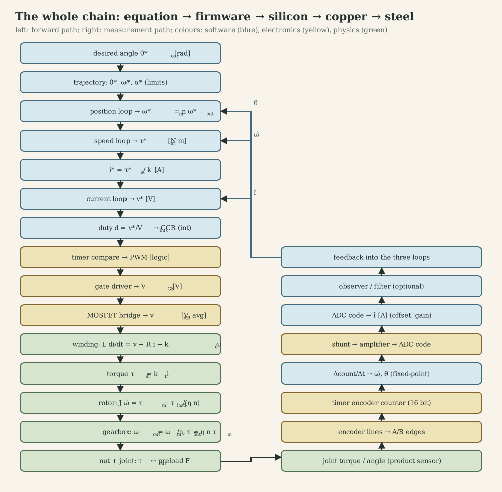
The table follows every arrow of the chain. Where numbers are needed, they come from the application drive of Part Q, the MF2030 nutrunner model (BX4 motor, $n=81$, 30 V battery, 20 kHz PWM, 10 kHz current loop, 1 kHz speed loop).
| # | Arrow | Physics and mathematics | Software and hardware representation | Limits and bandwidth | Noise, uncertainty, failure modes |
|---|---|---|---|---|---|
| 1 | Desired output angle / torque → trajectory | target 25 N·m, final speed 3 rad/s; angle window from joint stiffness | float targets in the tightening state machine; product parameters from comms |
speed and acceleration limits respect current and voltage limits | wrong joint parameters; no angle window (stripped threads go undetected) |
| 2 | Trajectory → position/angle loop | $\theta^\ast(t),\dot\theta^\ast,\ddot\theta^\ast$; P or PI on angle | thread at 100 Hz-1 kHz, k_timer |
bandwidth ≤ 1/5 of speed loop | trajectory not differentiable twice: feedforward spikes |
| 3 | Angle loop → speed reference | $\omega_m^\ast=n\,\omega_{\text{out}}^\ast$ (243 rad/s) | float, rad/s at the motor shaft (pick one shaft and stick to it) |
clamp at max speed (≈ 500 rad/s at 24-30 V) | output vs motor shaft confusion: factor 81 error |
| 4 | Speed loop → torque reference | PI: $K_p=0.072$ A·s/rad, $K_i=14.1$ A/rad (50 Hz, ζ = 0.8) | thread at 1 kHz woken by ISR | anti-windup; ~10× below current loop | quantized speed (1.5 rad/s per count at 1 kHz without a filter) |
| 5 | Torque → current reference | $i^\ast=\tau^\ast/k_t$ (7.9 A at clamp) | double-buffered float to the ISR |
clamp at peak current (e.g. 10 A) and by $I^2t$ thermal model | $k_t$ varies with temperature (magnets) and saturation |
| 6 | Current loop → voltage command | PI: $K_p=0.69$ V/A, $K_i=9.1\cdot10^3$ V/(A·s), plus back-EMF feedforward | ISR at 10 kHz, Tustin coefficients 1.147 / −0.236 | bandwidth ≈ 1 kHz; voltage clamp at $V_{\text{bus}}$ | one-sample delay costs 36° at 1 kHz; windup at voltage limit |
| 7 | Voltage → duty → compare value | $D=v^\ast/V_{\text{bus}}$; CCR $=D\cdot$ARR | uint16_t CCR; ARR = 2000 at 80 MHz centre-aligned |
duty 0-~95 % (bootstrap); 0.05 % resolution | stale $V_{\text{bus}}$ measurement: gain error; writing CCR without preload: glitches |
| 8 | Compare → PWM logic signals | timer compares counter with CCR | TIM1 hardware, complementary outputs | 20 kHz; dead time 500 ns (40 ticks) | dead-time error 0.24 V at 24 V; wrong polarity: shoot-through |
| 9 | Logic → gate voltage | gate driver sources/sinks amps; bootstrap for high side | driver IC, $C_{BS}$, gate resistors | switching times tens of ns | missing bootstrap refresh at high duty; ground bounce |
| 10 | Gate → bridge output voltage | switched $0/V_{\text{bus}}$; average $D\,V_{\text{bus}}$ | three-phase inverter (BLDC) or H-bridge (DC) | $V_{\text{bus}}$, $I_{\max}$, $T_j$ | ringing, EMI, body-diode conduction during dead time |
| 11 | Voltage → winding current | $L\,di/dt=v-Ri-k_e\omega$; $\tau_e=76$ µs | – | ripple 2.6 A p-p at 20 kHz, 1.3 A at 40 kHz | resistance rises with temperature; inductance with saturation |
| 12 | Current → electromagnetic torque | $\tau_m=k_ti$ (DC-equivalent) or $\tfrac32p\psi_mi_q$ | – | peak torque by current, continuous by heat ($\tau_{w1}=17$ s) | commutation ripple (six-step), wrong commutation angle |
| 13 | Torque → rotor acceleration | $J_i\dot\omega=\tau_m-\tau_{\text{load}}/(\eta n)$ | – | $\dot\omega_{\max}\approx k_ti_{\max}/J_i$ | friction (static 1.7 mN·m), unknown load |
| 14 | Rotor → gearbox → output | $\omega_{\text{out}}=\omega_m/n$, $\tau_{\text{out}}\approx\eta n\tau_m$ | – | gear torque rating; efficiency drops at light load | backlash, compliance (two-mass resonance), wear |
| 15 | Output → nut and joint | $\tau=F\,(p/2\pi+\mu_td_2/(2\cos30^\circ)+\mu_bD_b/2)$; $\approx32.6$ N·m/rad | – | bolt yield 640 MPa (class 8.8) | friction coefficient scatter ±30 %: same torque, different preload |
| 16 | Motion → encoder lines | $4N$ counts per revolution | quadrature A/B signals | max count rate of encoder and timer input filter | noise on long cables: false counts |
| 17 | Lines → timer counter | encoder mode counts edges | 16-bit TIMx->CNT |
wrap every 65 536 counts | direction reversed by wiring: positive feedback |
| 18 | Counter → speed and angle estimate | $\hat\omega=\Delta\text{cnt}\cdot2\pi/(N_{\text{cpr}}T_s)$ or Kalman filter | int16_t difference, float estimate |
quantum $2\pi/(N_{\text{cpr}}T_s)$ | delay of the estimator; wrong counts per revolution |
| 19 | Current → shunt voltage → ADC code | $v=R_Si$; amplifier gain and offset; 12-bit code | ADC injected conversion triggered by TIM1 | ±12 A full scale → 5.9 mA/LSB; sample at PWM centre | offset drift (torque ripple in FOC), saturation, wrong sampling instant (aliasing ripple) |
| 20 | ADC code → current estimate | $\hat i=(\text{code}-\text{offset})\cdot k_{\text{adc}}$ | float or Q15 |
calibrate offset at standstill with PWM off | uncalibrated offset → constant torque error |
| 21 | Torque transducer → stop decision | strain-gauge bridge in the output shaft | ADC + filter in the 1 kHz thread | decision delay ≤ 1 ms → 3 mrad at 3 rad/s | filter delay; transducer calibration traceability |
Two observations make this table useful in practice. First, every software representation is a unit and a range decision: rad/s or rpm, motor or output shaft, A or counts, Q15 or float. Most integration bugs are mismatches between two rows that were written by different people (exactly the “four teams” division of the MF2103 project). Second, bandwidths fall monotonically from the hardware outward (PWM 20 kHz, current 1 kHz, speed 50-100 Hz, angle 10 Hz); a requirement that violates this ordering cannot be met by tuning.
Part Q. Worked example: sizing a drive for a tightening application
This example applies the whole chain to one application, using the MF2030 simulation model (it was never built). The task, from the MF2030 assignment: tighten an M8 class 8.8 bolt to 25 N·m, ending the clamping phase at 3 rad/s at the nut, with the Faulhaber 3268 BX4 and the report’s two-stage gearbox ($n=81$). Labels: [D] datasheet, [M] modelled in MF2030, [R] re-derived here, [A] assumed, [C] design choice.
Q.1 Required output torque and speed
Target torque 25 N·m and final speed 3 rad/s at the nut [M]. How far does the nut turn while the torque rises? The MF2030 joint model ($T=k_{rs}\theta$, $k_{rs}=3.04$ N·m/rad) predicts 8.2 rad (470°) and a bolt stress of 3.4 GPa, impossible for a 640 MPa bolt. Including thread and under-head friction (VDI 2230 form, $\mu=0.2$ as in the report, $d_2=7.19$ mm, mean bearing diameter 11 mm [A]) gives
\[T=F\Big(\frac{p}{2\pi}+\frac{\mu d_2}{2\cos30^\circ}+\frac{\mu D_b}{2}\Big)=F\cdot2.13\ \text{mm},\]so 25 N·m produces a preload of 11.7 kN and a stress of 321 MPa (50 % of yield, a sensible tightening target), and only 9 % of the torque stretches the bolt. With the bolt stiffness alone, the nut turns about 44° from snug to target [R] (clamped parts in series make the joint softer, so the real angle is larger [unknown]).
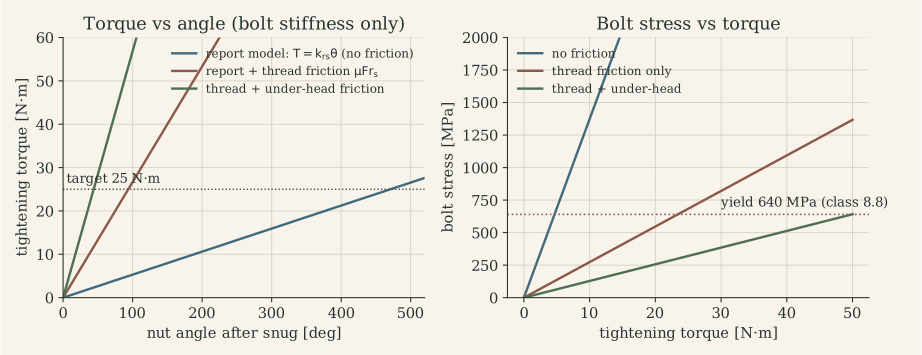
At 3 rad/s, 44° takes 0.26 s: the clamp phase is short, so the control loops must react within milliseconds.
Q.2 Map through the gearbox
\[\omega_m=n\,\omega_{\text{out}}=243\ \text{rad/s}\ (2320\ \text{rpm}),\qquad \tau_m=\frac{\tau_{\text{out}}}{\eta n}=\frac{25}{0.9\cdot81}=0.343\ \text{N·m},\]with $\eta=0.9$ for two planetary stages and the angle head [A]. Reflected output inertia $J_o/n^2=8.6\cdot10^{-10}$ kg·m² is negligible beside $J_i=6.2\cdot10^{-6}$ kg·m² [M]: the motor controller sees almost only its own rotor. The joint, seen from the motor, is a spring $k_T/n^2=5.0\cdot10^{-3}$ N·m/rad, which with $J_i$ resonates at 28 rad/s (4.5 Hz) [R]: slow compared with every control loop.
Is 81 the right ratio? The tightening requirement is a constant-power curve at the motor, $\tau_m\omega_m=75/0.9=83$ W, and every gear ratio picks a point on it (figure in B.7). The BX4’s peak power at 24 V is 99 W [D], so the clamp point is near the motor’s limit whatever the ratio. With $n=81$ the maximum nut speed is about 500/81 = 6.2 rad/s (59 rpm), so a 16-turn rundown takes 16 s; the product sheet’s 375 r/min free speed would need $n\le18.3$, where the clamp would require 1.52 N·m, twice the motor’s stall torque [D]. The assignment’s motor cannot meet both the product’s speed and torque: the real tool uses a larger motor, a shift strategy, or both [R].
Q.3 Motor torque and current
\[i=\frac{\tau_m}{k_t}=\frac{0.343}{0.0435}=7.9\ \text{A}.\]This is 5.6 times the continuous rating of 1.41 A [D]. Thermal check: copper loss $i^2R=90$ W; the winding’s thermal capacity $\tau_{w1}/R_{th1}=17/1.9=8.9$ J/K [D] gives an initial temperature rise of about 10 K/s, so a 0.26 s clamp adds about 3 K. The constraint is the RMS current over the work cycle: at full clamp current, the duty fraction must stay below $(1.41/7.9)^2\approx3$ %, for example one 0.26 s clamp every 8 s, ignoring rundown losses [R]. Firmware enforces this with an $I^2t$ model, not by trusting the operator.
Q.4 Required voltage
\[V=R\,i+k_e\omega_m=1.45\cdot7.9+0.0435\cdot243=11.4+10.6=22.0\ \text{V},\]plus about 0.2 V for two conducting MOSFETs at 10 mΩ [A] and a negligible $L\,di/dt$ in steady state. The headroom above 22 V determines how fast the current loop can change current: with 30 V, $di/dt\le8/110\,\mu\text{H}=7\cdot10^4$ A/s, so a 1 A correction takes 14 µs.
Q.5 Duty cycle
\[D=\frac{V}{V_{\text{bus}}}=\frac{22.2}{30}=0.74\quad(0.85\ \text{at a sagging 26 V pack [A]}).\]Measuring $V_{\text{bus}}$ and computing $D=v^\ast/V_{\text{bus}}$ keeps the current-loop gain independent of the battery state.
Q.6 Bridge switching
The BX4 is a three-phase BLDC motor: it needs a three-phase inverter, not the H-bridge of the lab boards. At 243 rad/s with $p=2$ the electrical frequency is 77 Hz; six-step commutation switches every 2.15 ms, each step driving one phase high and one low (I.2), with PWM on the active pair. Current ripple at 20 kHz:
\[\Delta I\approx\frac{V_{\text{bus}}D(1-D)}{L_{ll}f_{\text{PWM}}}=\frac{30\cdot0.74\cdot0.26}{110\,\mu\text{H}\cdot20\,\text{kHz}}=2.6\ \text{A p-p},\]a third of the average current. 40 kHz halves it to 1.3 A at twice the switching loss [C: 20 kHz with the ripple accepted, or 40 kHz if the switching loss permits].
Q.7 MCU peripheral configuration
On an STM32 with an advanced timer at 80 MHz [C]:
- TIM1 centre-aligned, ARR = 80 MHz / (2 · 20 kHz) = 2000; complementary outputs CH1/CH1N-CH3/CH3N; dead time 500 ns = 40 timer ticks (DTG); break input BKIN from the over-current comparator; outputs idle low on break or debug halt.
- TRGO at the counter peak triggers an ADC injected conversion of two phase currents (or the DC-link shunt for six-step) every second period (repetition counter = 1 → 10 kHz).
- Hall sensors on a timer in Hall-sensor interface mode (or three EXTI pins) for six-step sectors; encoder (if fitted) on another timer in encoder mode.
- ADC end-of-conversion interrupt at the highest priority for the current loop; bus voltage and the torque transducer on regular conversions.
Q.8 Sampling rates
| Loop | Rate | Bandwidth | Reason |
|---|---|---|---|
| Current | 10 kHz | 1 kHz | 10× above sampling rule; above any mechanical dynamics |
| Speed | 1 kHz | 50 Hz | 20× below current loop; joint resonance at 4.5 Hz is far below |
| Angle / torque supervision | 1 kHz | – | stop decision within 1 ms (3 mrad at 3 rad/s ≈ 0.1 N·m) |
| Trajectory, state machine | 100 Hz-1 kHz | – | phases last hundreds of ms |
| Communication, logging | asynchronous | – | tightening curves stored for traceability |
Q.9 Feedback control
- Current PI (on the DC-equivalent winding): $K_p=\omega_cL=0.69$ V/A, $K_i=\omega_cR=9.1\cdot10^3$ V/(A·s) for $\omega_c=2\pi\cdot1$ kHz, plus back-EMF feedforward $k_e\hat\omega$.
- Speed PI on $\beta=k_t/J_i=7015$ rad/s² per A: for 50 Hz and ζ = 0.8, $K_p=2\zeta\omega_0/\beta=0.072$ A·s/rad and $K_i=\omega_0^2/\beta=14.1$ A/rad.
- Tightening strategy. Speed control during rundown; when the transducer torque passes a threshold (snug), continue at clamp speed; stop on target torque. How much does the torque overshoot at the target? If the drive keeps commanding the clamp torque and lets the joint stop the rotor (a torque-limited stop), the rotor’s kinetic energy at 243 rad/s, $\tfrac12J_i\omega_m^2=0.18$ J, winds the joint (32.6 N·m/rad at the output) a further $\omega\sqrt{J_{\text{eq}}/k}=0.11$ rad: 3.5 N·m, 14 % overshoot from inertia alone [R]. Cutting the current exactly at 25 N·m is gentler, since the joint torque itself then brakes the rotor (about 0.2 N·m of overshoot), but it needs a fast, exact torque signal: at 3 rad/s every millisecond of measurement delay adds 0.1 N·m. Slowing to 0.5 rad/s at the nut before the target reduces the torque-limited overshoot to 0.6 N·m. This is the physical reason real nutrunners tighten in two steps (fast rundown, slow final approach) and brake actively at shut-off.
Q.10 Discretization
Tustin, incremental form:
\[u_k=u_{k-1}+q_0e_k+q_1e_{k-1},\qquad q_0=K_p+\tfrac{K_iT_s}{2},\quad q_1=-K_p+\tfrac{K_iT_s}{2}.\]Current loop ($T_s=100$ µs): $q_0=1.147$, $q_1=-0.236$. Speed loop ($T_s=1$ ms): $q_0=0.0787$, $q_1=-0.0646$. The current loop’s computation-plus-PWM delay (0.5-1.5 periods) costs 18-54° at 1 kHz: either include $z^{-1}$ in the design, or lower the bandwidth to about 600 Hz. Position-form implementations need explicit anti-windup; the incremental form is naturally bounded if $u$ is clamped before it is stored.
Q.11 Sensing noise
- Current: ±12 A full scale [C] on a 12-bit ADC is 5.9 mA per LSB. A noise of 20 mA corresponds to 0.9 mN·m at the motor, 0.06 N·m at the nut: 0.25 % of the target.
- Speed: an encoder with 4096 counts/rev [A] at 1 kHz gives 1.53 rad/s quantization at the motor; a Kalman filter (H.3) brings the estimate’s standard deviation to about 0.07 rad/s.
- Torque transducer: its noise and calibration set the final accuracy; values are not in the course material [unknown]. Production tools are verified against external reference transducers.
Q.12 Delay and jitter budget
| Path | Delay | Jitter | Effect |
|---|---|---|---|
| ADC trigger → ISR start | 2-4 µs (conversion + entry) | < 1 µs (hardware triggered) | negligible |
| ISR execution (FOC or current PI) | 15-25 µs WCET [A] | branch-dependent, a few µs | must finish before the update event |
| Sample → new duty active | 0.5-1.5 PWM periods (25-75 µs) | fixed by hardware | include in current-loop design |
| Speed thread start after 10th ISR | ≤ 1 ISR WCET | ≤ 25 µs | negligible at 1 kHz |
| Torque threshold → shut-off | ≤ 1 ms | ≤ 1 ms | 3 mrad, ≈ 0.1 N·m |
Q.13 RTOS execution structure
The Zephyr architecture of N.7: TIM1 and ADC in hardware; the current loop in a direct ISR; the speed loop, torque supervision and tightening state machine in a cooperative thread at 1 kHz woken by the ISR; trajectory and parameters in a 100 Hz thread; Bluetooth/radio communication and storage of tightening curves in low-priority threads fed by message queues. Utilization is about 0.4 with the WCETs of M.3.
Q.14 Safety limits
- Peak current clamp (10 A) in the current loop, hardware over-current break on TIM1 BKIN.
- $I^2t$ thermal model with $\tau_{w1}=17$ s and $\tau_{w2}=1060$ s; derate the current limit when the model temperature rises.
- Torque limit 110 % of target and angle window (for example 20-90° after snug [A]) to reject stripped threads, missing washers or cross-threading.
- Stall detection: high current with low speed during rundown for more than about 50 ms means a jam.
- Reaction torque: in a hand-held tool, the operator absorbs the reaction; limit the torque rise rate and brake at shut-off.
- Bus over-voltage during braking (regeneration into the battery, J.4); under-voltage cut-off for the pack.
- Watchdog; on any fault, outputs off in hardware first, then report.
Q.15 Bring-up and debugging plan
- Power stage on a resistive load; check gate signals, dead time and switch node on a scope (O.3).
- Open-loop six-step at low duty; verify the Hall-to-step table by direction and current waveform (I.2).
- Current loop on a blocked rotor; step response of the current from the shunt; check sign and offset.
- Speed loop without load; step and reversal; check anti-windup by holding the shaft (the MF2103 lesson).
- Joint simulator (a spring-loaded test joint) with a reference torque transducer; tune the two-step tightening and measure overshoot.
- Timing verification: GPIO toggles in ISR and threads; worst case with communication and logging active.
- Fault injection: disconnect the encoder, short a phase through a current-limited supply, drop the bus voltage; verify each protection reaction.
Q.16 What the example teaches
The decisive numbers came from different disciplines: friction (mechanics) sets the angle and preload; the constant-power curve (machine physics) exposes the gear-ratio conflict; RMS current (thermal) bounds the work cycle; rotor kinetic energy (dynamics) dictates a two-step control strategy; current ripple (power electronics) argues for a higher PWM frequency; delay (real-time) limits the current-loop bandwidth; and fixed-point ranges (embedded C) decide whether the controller survives a stalled rotor. None of these is visible from inside one discipline.
References and reading guide
My course material and artefacts (documented on the project page):
- MF2030 Mechatronics basic course (KTH, HT21): lecture C2 “Modeling and analysis of mechatronic actuators, especially PMSM machines”; lectures 4-6 (DC motor case, transducers, implementation); lecture 9 (multibody and linear electrical actuators); project “An Electric Nut-Runner for Tightening of Bolted Joints” (Group 2: G. R. Rangaraju, X. Niu, P. C. Hau).
- MF2007 Dynamics and Motion Control (KTH, 2021-22): chapters C1-C7 (modelling, actuators, feedback, discrete control, servo control, implementation, robustness); Workshops A and B, group 4 (X. Niu, H. Chen, J. Wang).
- MF2043 Mechatronic Electronics (KTH, HT21): lectures on power supplies, actuator and sensor interfaces, filters, EMC, transients, troubleshooting; labs 1-4 (supply, H-bridge, anti-alias filters, current sensor), designs in Eagle.
- MF2103 Embedded Systems for Mechatronics (KTH, VT22): seminars on embedded computing, RTOS and distributed systems; tutorials 1-5; project tasks 0-3.
- 1DT106 Programming Embedded Systems (Uppsala University, 2025): lectures 1-10 and Zephyr examples, github.com/uu-pes.
Books and articles:
- K. Janschek, Mechatronic Systems Design (Springer, 2012). Transducers, multibody models, mechatronic modelling (MF2030 course book).
- A. Hughes and B. Drury, Electric Motors and Drives (5th ed., Newnes, 2019). Physical understanding of all machine types.
- R. Krishnan, Permanent Magnet Synchronous and Brushless DC Motor Drives (CRC, 2010).
- N. Mohan, Electric Machines and Drives: A First Course (Wiley, 2012); N. Mohan, T. Undeland, W. Robbins, Power Electronics (Wiley, 2003).
- H. E. Merritt, Hydraulic Control Systems (Wiley, 1967); P. Beater, Pneumatic Drives (Springer, 2007).
- K. J. Åström and B. Wittenmark, Computer-Controlled Systems (3rd ed., Prentice Hall, 1997). Sampling, discretization, delay and jitter.
- G. F. Franklin, J. D. Powell, M. Workman, Digital Control of Dynamic Systems (3rd ed., Addison-Wesley, 1998).
- K. J. Åström and T. Hägglund, Advanced PID Control (ISA, 2006). Anti-windup, set-point weighting, derivative filtering.
- D. Simon, Optimal State Estimation: Kalman, H-infinity, and Nonlinear Approaches (Wiley, 2006).
- R. B. Northrop, Introduction to Instrumentation and Measurements (3rd ed., CRC, 2014). Sensors, amplifiers, noise.
- W. Kester (ed.), The Data Conversion Handbook (Analog Devices / Newnes, 2005). Sampling, aliasing, ADC and DAC architectures.
- G. C. Buttazzo, Hard Real-Time Computing Systems (3rd ed., Springer, 2011). RMS, EDF, response-time analysis.
- J. Yiu, The Definitive Guide to ARM Cortex-M3 and Cortex-M4 Processors (3rd ed., Newnes, 2014). Exceptions, stacking, fault handling.
- T. Martin, The Designer’s Guide to the Cortex-M Processor Family (Newnes); W. Wolf, Computers as Components, ch. 1 (MF2103 readings).
- H. W. van der Broeck, H.-C. Skudelny, G. V. Stanke, “Analysis and Realization of a Pulsewidth Modulator Based on Voltage Space Vectors,” IEEE Trans. Industry Applications 24(1), 1988.
- J. C. Doyle, “Guaranteed Margins for LQG Regulators,” IEEE Trans. Automatic Control 23(4), 1978.
- VDI 2230 Part 1, Systematic calculation of highly stressed bolted joints (VDI, 2015).
Datasheets and documentation: Faulhaber 3268 G 024 BX4 brushless DC-servomotor datasheet; Assun AM-CL1643MB-1210 coreless DC motor datasheet; Allegro A4973 full-bridge PWM motor driver; TI LM2576, LM317, INA126; STMicroelectronics RM0351 (STM32L4 reference manual) and UM1724 (Nucleo-64); Atlas Copco Tensor STB product sheets; Zephyr Project documentation (kernel services, devicetree, nucleo_l476rg and wiznet_w5500 board pages).
Figures: diagrams and plots are my own (simulations re-run in Python from the course models and code). Photos: Zephyr Project documentation (Nucleo-L476RG pinout, Apache-2.0); Wikimedia Commons (C2000 LaunchPad by Brihaspati, CC BY-SA 4.0; floppy-drive spindle motor by Sebastian Koppehel, CC BY 3.0).